Download
1 / 80
880 likes | 1.86k Vues
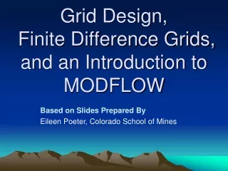
Grid Design, Finite Difference Grids, and an Introduction to MODFLOW. Based on Slides Prepared By Eileen Poeter, Colorado School of Mines. Conceptual Model Defines . 1) Dimensions of numerical model 2) How the grid is designed 3) How the grid is oriented. Representation of Numerical Model.

E N D
Grid Design, Finite Difference Grids, and an Introduction to MODFLOW Based on Slides Prepared By Eileen Poeter, Colorado School of Mines
Conceptual Model Defines • 1) Dimensions of numerical model • 2) How the grid is designed • 3) How the grid is oriented
DISCRETIZED HYPOTHETICAL AQUIFER Layers may correspond to horizontal geohydrologic intervals ---- Aquifer boundary ● Active cell ○ Inactive cell Δrj Width of cell in row direction (j indicates column number) Δci Width of cell in column direction (i indicates row number) Δvk Thickness of the cell ΔrjΔciΔvk Volume of cell with coordinates (i,j,k)
Representation of Numerical Model • Choose numbers to define a conceptual object like the grid shown below to represent the geometry, properties, boundary conditions, initial conditions and stresses on a groundwater system to build a representation of field conditions Videos of Flow (Mojave, Santa Clara Transport Models (Tracy?)
Representation of Numerical Model • Divide space into pieces • Define one value for each geohydrologic parameter to represent the piece • One value defined for each physical property (ie. K and S) • One value of head and flow is calculated • Complex geologic material distributions are simplified • Properties vary • Within a layer • From layer to layer
Representation of Numerical Model • Some of the model pieces are defined as inactive (open circles) • Take the rectangular form of the mathematics and create an odd shaped geometry • Inactive indicators may continue down through every layer of the grid, or not Example: aquifer is bowl shaped then some pieces that are active in the shallow layers would be specified as inactive in the deeper layers
Grid Design • Numerical model needs to be divided into pieces of space and time for which the solution can be linearized and the properties and results averaged • Compromise between accuracy, cost, and effort • Smaller pieces are more accurate, but require more time and effort
Grid Design • Discretize: • Space (plan view and cross section) • Time • Difficult Task • Redesign is a major undertaking
Spatial Dimension • 2D areal • 2D profile (special class) • Quasi 3D (confining layers by leakage) • Fully 3D • Aquifer viewpoint: 2D areal and quasi 3D • Flow system viewpoint: 2D profile and 3D
QUASI THREE DIMENSIONAL Flowlines in sand are nearly horizontal Flowlines in clay are nearly vertical Quasi-3d Single model layer maybe used to represent each sand, while the clay may be represented by the vertical conductance between layers Clay layer is represented by six model layers. Use if clay storage is an issue.
Fully 3D Models • Simulate confined and unconfined aquifers when vertical head gradients are important • Represent transient release of water from storage in confining beds by including confining bed as a layer with storage properties • Parameter arrays specified for each layer of the model
Parameters • Transmissivity • Hydraulic conductivity • Thickness • Anisotropy • Storage properties
Laying out the grid • Types of Grids • Defining Model Layers • Orienting the Grid • Spatial Scales
Types of Grids • Array of Nodes • Grid Structure • Finite elements • Finite difference cells
Finite Elements • Allow more flexibility in designing grid • 2D elements • Triangles • Quadrilaterals • 3D elements • Tetrahedrons • Hexahedrons • Prisms • Exact representation of boundaries is possible • Input of data is generally more laborious than finite difference
Finite difference cells • Mesh-centered • Block-centered • Easier math for boundaries • MODFLOW
Defining Model Layers • One layer • layer represents a single hydrostratigraphic unit or aquifer • Quasi-3D • Hydrogeologic units horizontal • Leakance • Fully 3D • Dipping units • Aquifers and Confining units explicit
Orienting the Grid • Grid drawn on an overlay of a map of the area to be modeled • If possible orient the grid so that the x and y axes are colinear with Kx and Ky and vertical axis is aligned with Kz • For finite difference, try to minimize the number of nodes that fall outside the boundaries of the modeled area • Set boundaries far from the area of interest so imposed stresses to the interior of system don’t reach the boundaries
Spatial Scales • Critical Step • Based on: • Size of model area • Changes in head (primary) • Changes in aquifer properties (secondary) • Changes in recharge, pumping, surface-water interaction
Spatial Scales • Horizontal Node Spacing: • Function of expected curvature in the water table or potentiometric surface • Variations in aquifer properties in horizontal dimension typically greater than vertical • Vertical Node Spacing: • Function of change in head in the vertical direction • Typically one layer per hydrostratigraphic unit • Significant vertical head gradients may want more
Vertical discretization can vary depending on use of the model Halford, 1999
Spatial Scales • Overall size of model area also affects the selection of model area • Compromise between accuracy and practicality • Small number of nodes • Minimize data handling, computer storage and computation time • Large number of nodes • Represent system accurately • Meaningful boundaries may require a large area
Variably spaced finite-difference grid allows good discretization of remediation area, while allowing model to go to hydrologic boundaries. Halford, 1999
Assigning Parameter Values • Data Needs (Discussed last week) • Two Categories • Physical framework (geometry including thickness, extent, and properties of units) • Hydraulic data (heads and fluxes) • Transferring field data to the grid • Scale issues • Zones (sets of nodes with similar properties) • Interpolation algorithms such as kriging • Hydrogeologic judgement • WHATEVER METHOD, DISTRIBUTIONS MUST BE REASONABLE AND MAKE SENSE!!!!
FINITE DIFFERENCE METHOD The continuous system is replaced by a finite set of discrete points in time and space The partial derivatives are replaced by terms calculated from the differences in head values at these points The discretization process results in a system of simultaneous linear algebraic equations—difference equations The solution to the difference equations yields values of head at specific points and time
Finite Difference MethodsSee handout taken from Lessons Prepared ByEileen Poeter, Colorado School of Mines • Spreadsheet Example • MODFLOW
Discretize Time and SpaceFINITE DIFFERENCE AND MODFLOW • Plan View • Cross Sectional View • Time
Discretize Time and Space • Plan View • For a finite-difference grid, lines between cells need to orthogonal and extend the entire width of the grid • any detail defined in the interior of the grid is extended all the way to the edges • most finite-difference codes allow the width of cells along rows to vary
Plan View Grid Considerations • Problem Domain • External Inactive Grids • Flow Direction • Anisotropy • Minimize Number of Cells • Boundaries Between Features • Stress Areas • Observation Points • Symmetry • Relative Size of Adjacent Grids (1.5) • Orthogonal Directions (100:1) • Future Solute Transport
Plan View Grid Considerations • Problem Domain • Use well-defined, permanent natural boundaries when possible. • If a boundary is not permanent (e.g. a ground-water divide) anticipate potential future variations, and either accommodate them from the start or be prepared to monitor appropriately and make adjustments later. • Most approaches to grid development require substantial time and effort to make substantial changes to the model grid.
Plan View Grid Considerations • External Inactive Grids • Rotate grid to allow as few nodes as possible outside the active model domain • Minimize input and output file size • Make data management easier • Flow Direction • Orient grid so that the primary flow direction is aligned with the rows and columns • Flow calculations are oriented along rows and columns, so diagonal flows are calculated in a stair-step manner, thus orienting the rows and columns in the direction of flow will reduce errors.
Plan View Grid Considerations • Anisotropy • Orient grid so that the rows and columns of the grid coincide with the major axes of the hydraulic conductivity ellipsoid. • Minimize Number of Cells • Easier to manage • Executes more quickly • Tradeoff with accuracy • Boundaries Between Features • More detailed grid where conditions change abruptly • May need gradual transition in parameter values at a contact, which can reduce calculation errors or convergence trouble. If the cells are small, such a gradation is a fairly good approximation of the actual transition.
Plan View Grid Considerations • Stress Areas (Steep Gradients) • Gradient between cells represented by a straight line. • Better solution if many small cells are used. • Observation Points / Areas of Interest • Head, concentration, or flow rate can be interpolated between cells • More accurate and more convenient to have cells at needed locations • Symmetry • May allow you to cut your model size in half or more • Common when simulating engineered features • Relative Size of Adjacent Grids (1.5) • Orthogonal Directions (100:1) • Future Solute Transport
Plan View Grid Considerations • Relative Size of Adjacent Grids (1.5) • If adjacent grids have substantially different size, then truncation errors may occur in the matrix solution. • To avoid problems maintain a maximum size difference of 1.5 for adjacent cells. • Orthogonal Directions (100:1) • Aspect ratio is less critical than relative size. • Acceptable for the ratio of length to width, or width to length, to be 100:1. • Future Solute Transport • Frequently requires much smaller cells than flow modeling • Often advantageous to start with this discretization
Discretize Time and Space • 2) Cross Sectional View • MODFLOW allows thickness of layers to vary on a cell by cell basis • Each layer must extend across the entire model • Pinch outs must be dealt with by changing properties of the layer
Layer Considerations • One Layer = NO VERTICAL flow, flow parallel to layer • Vertical Components = stacks of cells, layers • Two layers = upward or downward gradient of one magnitude (cannot calculate convergent flow) • Complicated vertical flow patterns = multiple layers
Layer Considerations • Purpose of Model • Regional vs. Local • Partial Penetration • Confining Unit Storage • Future Transport Modeling • Hydrostratigraphic Units • Geologic Logs • Geophysics • Vertical Hydraulic Gradients • Dewatering • Layer Representation Options • Constant layer thickness (variable properties) • Variable layer thickness (constant properties) • Relative size of adjacent grids is not an issue in vertical direction
Layer Considerations – Purpose of the Model • Regional vs. Local • Units likely to be grouped or lumped in regional • More detail in local • Nature of question will influence • Partial Penetration • Layers to define open interval • Additional layers to define head gradients and flow paths • Confining Unit Storage • Future Transport Modeling
Layer Considerations – Purpose of the Model • Confining Unit Storage • No layers • No storage • Leakage • Multiple layers • Water in storage • Long travel times for pressure gradient • Future Transport Modeling • All of above issues • Travel time requires multiple layers No cells for confining unit: Multiple layers for confining unit:
Layer Considerations (cont.) • Hydrostratigraphic Units • Geologic Logs • Build a 3D stratigraphy • Determine lumping/simplification • Even homogeneous may have vertical gradients because of boundaries • Geophysics • Use to add to information from geologic logs • Vertical Hydraulic Gradients • Determine if natural gradients are important to your problem • Enough layers to represent variation in gradients
Layer Considerations (cont.) • Dewatering • The original version of MODFLOW would not allow grid cells to "re-wet" if the head had dropped below the bottom of a cell in a previous iteration. These cells would become impermeable. The modern MODFLOW accommodates this feature. However there are often convergence issues or long run times. • If not using rewetting, you may have to make shallow units thick in order to keep them from completely dewatering. Of course, this means that you will not evaluate vertical components of flow in that zone.permanently impermeable zone if re-wetting option is not used, even if the well is turned off:
Layer Considerations (cont.) • Relative size of adjacent grids is not an issue in vertical direction • MODFLOW connects layers explicitly, consequently you do not need to be concerned about truncation errors in a matrix solution for vertically adjacent cells.
Layer Considerations (cont.) • Layer Representation Options • Constant layer thickness /variable properties • Expedites modeling • Rough approximation • Compatibility with another function • Variable layer thickness /constant properties • More representative of field conditions
Discretize Time and Space • 3) Discretize Time • TIME STEPS: temporal equivalent of grid cells • Small when stresses change and increase in length to a constant, convenient size until the stresses change • STRESS PERIODS: groups of time steps during which stresses do not change • Temporal data compiled at these increments
Time Discretization Considerations • Difficult to decide on initial time step size • MODFLOW requires the time period, number of steps and a multiplier to gradually increase steps Multiplier is typically 1.1 to 1.5
How small is small enough? • YOU KNOW YOUR DISCRETIZATION IS APPROPRIATE WHEN: • THE ANSWER REMAINS THE SAME FOR:SMALLER TIME STEPS, STRESS PERIODS,ANDSMALLER CELL SIZES • TIME • Easy to test smaller time steps • Stress periods require recompiling stress data (may be time consuming) and updating any packages with stresses specified • SPATIAL • Unless you have an automated grid generator / input file creator, then the time requirements and logistics of rebuilding the model with smaller cell sizes renders the task unreasonable • Important to use smaller grid sizes from the beginning of numerical model development because you will never be able to test this issue. • In reality, few if any modelers check this.
MODFLOW • MODFLOW is the world's most used ground-water modeling code • Goal was/is to be: • easy to understand, • use, and • modify
Versions of MODFLOW Trescott, Pinder, and Larson codes MODFLOW (much longer name) MODFLOW-88 (first version) MODFLOW-96 MODFLOW-2000 MODFLOW-2005 This class will use the documentation for MODFLOW-2005 as a primary reference. Class projects will be done with this version. The report and program can be downloaded to your computer from USGS web site http://water.usgs.gov/nrp/gwsoftware/modflow2005/modflow2005.html