Download
1 / 21
210 likes | 359 Vues
-1. 1. 2. 3. 2. 4. 8. 9. 10. 9. 1. -1. 2. 4. 1. 1. -1. 0. Other Edge Detection Filters. Another idea for edge detection is to use the magnitude of the first derivative of the intensity function as a measure for edge strength.

E N D
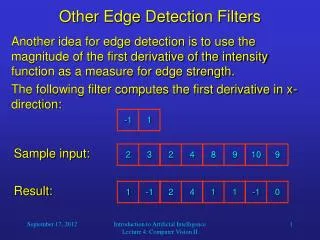
-1 1 2 3 2 4 8 9 10 9 1 -1 2 4 1 1 -1 0 Other Edge Detection Filters • Another idea for edge detection is to use the magnitude of the first derivative of the intensity function as a measure for edge strength. • The following filter computes the first derivative in x-direction: Sample input: Result: Introduction to Artificial Intelligence Lecture 4: Computer Vision II
Other Edge Detection Filters • As you probably noticed, one problem with this filter is that it has no center element that would point to the position for which the derivative is computed. • Also, a filter that only covers two pixels at a time may produce very noisy results. • In order to solve these problems, we can use a pair of 33 filters instead (one for x- and one for y- direction). • One such solution is called the Sobel filter. Introduction to Artificial Intelligence Lecture 4: Computer Vision II
-1 0 1 1 2 1 -2 0 2 0 0 0 -1 0 1 -1 -2 -1 Sx Sy Sobel Filters • Sobel filters are another variant of edge detection filters. • Two small convolution filters are used successively: Introduction to Artificial Intelligence Lecture 4: Computer Vision II
sy sx Other Edge Detection Filters • Consider the magnitudes of the sx and sy outputs for edges of different orientations: Introduction to Artificial Intelligence Lecture 4: Computer Vision II
Sobel Filters • Sobel filters yield two interesting pieces of information: • The magnitude of the gradient (local change in brightness): • The angle of the gradient (tells us about the orientation of an edge): Introduction to Artificial Intelligence Lecture 4: Computer Vision II
Result of calculating the magnitude of the brightness gradient with a Sobel filter Sobel Filters Introduction to Artificial Intelligence Lecture 4: Computer Vision II
-1 1 Computation of the Second Derivative • Let us now return to the computation of the second derivative, as needed for the Laplacian edge detection method. • As you know, the second derivative is the “rate of change” in the first derivative along the x- or y-axis. • So the basic idea for computing the derivative along the x-axis is to use the minimal filter and apply it at two consecutive x-positions. The same filter is then applied to the two resulting values, yielding the second derivative. Introduction to Artificial Intelligence Lecture 4: Computer Vision II
a b c a b c 2 2 4 4 5 5 … … -1 -1 -2 -1 1 1 1 1 1 2 1 -a + b -b + c 0 -1 … … 0 -1 … … a - 2b + c Computation of the Second Derivative Implemented as single convolution: same result! Introduction to Artificial Intelligence Lecture 4: Computer Vision II
0 0 0 0 1 0 0 1 0 1 -2 1 0 -2 0 1 -4 1 + = 0 0 0 0 1 0 0 1 0 x-filter y-filter xy-filter Computation of the Second Derivative • The 2D derivative can then be computed as the sum of the x- and y-derivatives: The resulting filter is identical to the 33 Laplacian filter that we discussed last week. Introduction to Artificial Intelligence Lecture 4: Computer Vision II
Object Recognition • How can we devise an algorithm that recognizes objects? • Problems: • The same object looks different from different perspectives. • Changes in illumination create different images of the same object. • Objects can appear at different positions in the visual field (image). • Objects can be partially occluded. • Objects are usually embedded in a scene. Introduction to Artificial Intelligence Lecture 4: Computer Vision II
Object Recognition • We are going to discuss an example for view-based object recognition. • The presented algorithm (Blanz, Schölkopf, Bülthoff, Burges, Vapnik & Vetter, 1996) tackles some of the problems that we mentioned: • It learns what each object in its database looks like from different perspectives. • It recognizes objects at any position in an image. • To some extent, the algorithm could compensate for changes in illumination. • However, it would perform very poorly for objects that are partially occluded or embedded in a complex scene. Introduction to Artificial Intelligence Lecture 4: Computer Vision II
The Set of Objects • The algorithm learns to recognize 25 different chairs: It is shown each chair from 25 different viewing angles. Introduction to Artificial Intelligence Lecture 4: Computer Vision II
The Algorithm Introduction to Artificial Intelligence Lecture 4: Computer Vision II
The Algorithm • For learning each view of each chair, the algorithm performs the following steps: • Centering the object within the image, • Detecting edges in four different directions, • Downsampling (and thereby smoothing) the resulting five images. • Low-pass filtering of each of the five images in four different directions. Introduction to Artificial Intelligence Lecture 4: Computer Vision II
The Algorithm • For classifying a new image of a chair (determining which of the 25 known chairs is shown), the algorithm carries out the following steps: • In the new image, centering the object, detecting edges, downsampling and low-pass filtering as done for the database images, • Computing the difference (distance) of the representation of the new image to all representations of the 2525 views stored in the database, • Determining the chair with the smallest average distance of its 25 views to the new image (“winner chair”). Introduction to Artificial Intelligence Lecture 4: Computer Vision II
x 1 2 3 4 5 1 2 y 3 4 5 The Algorithm Compute the center of gravity: • Centering the object within the image: • Binarize the image: Finally, shift the image content so that the center of gravity coincides with the center of the image. Introduction to Artificial Intelligence Lecture 4: Computer Vision II
Object Recognition • Detecting edges in the image: • Use a convolution filter for edge detection. • For example, a Sobel filter would serve this purpose. • Use the filter to detect edges in four different orientations. • Store the resulting four images r1, …, r4 separately. Introduction to Artificial Intelligence Lecture 4: Computer Vision II
Object Recognition • Downsampling the image from 256256 to 1616 pixels: • In order to keep as much of the original information as possible, use a Gaussian averaging filter that is slightly larger than 1616. • Place the Gaussian filter successively at 1616 positions throughout the original image. • Use each resulting value as the brightness value for one pixel in the downsampled image. Introduction to Artificial Intelligence Lecture 4: Computer Vision II
Object Recognition • Low-pass filtering the image: • Use the following four convolution filters: • Apply each filter to each of the images r0, …, r4. • For example, when you apply k1 to r1 (vertical edges), the resulting image will contain its highest values in regions where the original image contains parallel vertical edges. Introduction to Artificial Intelligence Lecture 4: Computer Vision II
Object Recognition • Computing the difference between two views: • For each view, we have computed 25 images (r0, …, r4 and their convolutions with k1, …, k4). • Each image contains 1616 brightness values. • Therefore, the two views to be compared, va and vb, can be represented as 6400-dimensional vectors. • The distance (difference) d between the two views can then be computed as the length of their difference vector:d = || va – vb || Introduction to Artificial Intelligence Lecture 4: Computer Vision II
Results • Classification error: 4.7% • If no edge detection is performed, the error increases to 21%. • We should keep in mind that this algorithm was only tested on computer models of chairs shown in front of a white background. • The algorithm would fail for real-world images. • The algorithm would require components for image segmentation and completion of occluded parts. Introduction to Artificial Intelligence Lecture 4: Computer Vision II