Understanding Enzyme Reactions and Molecular Machines
460 likes | 536 Vues
Explore enzyme reactions, molecular machines, and modulation of enzyme activity, including an overview of catalysis, enzyme kinetics, and recent developments. Discover the intriguing world of molecular motors and membrane protein translocation.

Understanding Enzyme Reactions and Molecular Machines
E N D
Presentation Transcript
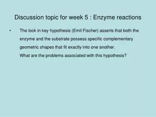
Discussion topic for week 5 : Enzyme reactions • The lock in key hypothesis (Emil Fischer) asserts that both the enzyme and the substrate possess specific complementary geometric shapes that fit exactly into one another. What are the problems associated with this hypothesis?
Enzymes and Molecular Machines (Nelson, chap. 10) Enzymes are biological catalysts that enhance the rate of chem. reactions. Machines use free energy from an external source (e.g. ATP, concentration or potential difference) to do useful work. Examples: • Motors: transduce free energy into linear or rotary motion • myosin on actin in muscles, kinesin on microtubules in cells. • Pumps: create concentration differences across membranes • sodium-potassium pump transports 3 Na+ ions out of the cell and 2 K+ ions into the cell in one cycle. • Synthases: drive chemical reactions to synthesize biomolecules • ATP synthase synthesizes the ATP molecules that are used by most of the molecular machines in the cells.
Enzymes An extreme example: catalese Consider the decomposition of hydrogen peroxide: H2O2 H2O + ½ O2 DG0 = -41 kT so the reaction is highly favoured but due to a high activation barrier it proceeds very slowly: for 1 M solution the rate is 10-8 M/s (reaction velocity) Adding 1 mM catalese into the solution increases the rate by 1012 ! 10-3 NA catalese molecules perform 104NA hydrolisis reactions per sec. So 1 catalese molecule catalyses 107 reactions per sec. (rate: 10-7 s) H2O2 is produced in cells while eliminating free radicals. Because it is toxic, its rapid breakdown is important. More typical rates for enzymes are around 103 s-1
Simple model of enzyme reactions: Chemical reactions involving biomolecules are extremely complex. Free energy surface typically involves thousands of coordinates. Nevertheless a reaction usually proceeds along the path of least resistance (called reaction coordinate) which allows a simple description. transition state A simple reaction: H + H2 H2 + H
An enzyme facilitates a chemical reaction by binding to the transition state and thereby reducing the activation energy, DG‡ (but not DG) Free energy surface along the reaction coordinate DG‡ DG‡ DG DG Substrate Enzyme + substrate
Direction of the reaction is controlled by DG. By changing DG, we can reverse the direction. The reverse reaction does not necessarily follow the same reaction coordinate.
A schematic picture of an enzyme E binding to a substrate S: E + S ES EP E + P E+S: The enzyme has a binding site that is a good match for the subst. S ES: In order to bind, S must deform which stretches a bond to breaking pt. EP: Thermal fluctuations break the bond producing an EP complex E+P: The P state is not a good match to the binding site, hence it unbinds, leaving the enzyme free for binding of the next substrate.
Corresponding free energy surface
Enzyme Kinetics: Consider an enzyme reaction with rate constants k1, k2 and k3 Assume: For a single enzyme, the reaction simplifies to Let probability of E unoccupied be PE and occupied PES = (1- PE) The rate of change of PE is
Assuming quasi-steady state, the time derivative vanishes, yielding Rate of production of P per enzyme: Reaction velocity for a concentration cE of enzymes Michaelis-Menten (MM) rule
Experimental data for pancreatic carboxypeptidase vmax=0.085 mM/s KM=6.4 mM
MM rule displays saturation kinetics, which has very general validity The key idea is the processing time for S P At low substrate concentrations, there are more enzymes than S so that there is no waiting and hence v is proportional to cS As cS is increased beyond KM, there is competition among S for access to an enzyme, and they have to queue for processing. Maximum velocity of the reaction is determined by the number of enzymes available and the processing rate (the rate limiting step) Modulation of enzyme activity: • Regulate the rate of enzyme production • Competitive inhibition: direct binding of another molecule • Noncompetitive inhibition: binding of a molecule to a second site
Recent developments (Adenylate kinase) We know very little about the actual dynamical processes occurring in enzymes. There are only a few simple cases where the physical mechanism is understood, e.g. oxygen binding in myoglobin. Adenylate kinase catalyzes: ADP + ADP ATP + AMP Recent work indicates that the rate limiting step is the enzyme conformation, and not the chemistry.
Molecular motors in muscles: myosin and actin For structure of the myosin and actin filaments in a myofibril, see http://distance.stcc.edu/AandP/AP/AP1pages/Units5to9/Unit7/myofibri.htm Experiment with optical tweezers demonstrates how myosin pulls an actin filament when 1 mM of ATP is added to the system. From Finer et al. “Single myosin molecule mechanics” Nature, 1994.
Translocation of proteins across membrane: Proteins produced in the cell are exported outside through proteins in the membrane that form pores. To pass through the pore, the protein has to unfold. The reverse motion is suppressed because the chemical asymmetries between inside and outside of the cell leads to a more stable protein structure outside. Factors contributing to asymmetry: • pH • ion concentration • disulfide bonding • binding of sugars protein catalyzes translocation
Macroscopic machines are deterministic, there are no random fluctuations But molecular machines operate in a noisy environment with lots of random fluctuations. Consider the ratchets below as possible models for molecular machines. In G-ratchet the spring retracts during the passage but pops back after In S-ratchet a latch releases the spring after the passage, which stays up Can either ratchet pull a load f towards right doing useful work?
Unloaded G-ratchet makes no net motion, the loaded one moves to the left S-ratchet moves to the right if e > f.L, and to the left if e < f.L (no net motion if e = f.L)
Simple model for a perfect Brownian ratchet: (e >> kT) In the absence of any forces, the ratchet diffuses freely until it travels a distance L. From Thus the average speed is: Next we introduce a load f that pulls the ratchet to the left. The potential energy increases as in the interval [0, L] From Boltzmann distribution, the equilibrium probability will be like
We need an equation to describe the nonequilibrium probability distribution of the ratchet’s position (cf. Fick’s law and Nerst-Planck Eq.) | | | | | x Dx >> L a-Dx/2 a a+Dx/2 a+Dx The net flux from a a+Dx depends on (1) the probabilities at those points and (2) the external forces. If there are N ratchets in our ensemble, the bins at a and a+Dx have ratchets. Assuming they move randomly, the net migration from left to right is
Next consider the flux due to an external force, Drift velocity due to this force: The number of ratchets moving from left to right: Adding the two contributions and dividing by Dt, we obtain for the flux Steady state: flux is constant, and from continuity eq. it is also uniform (Smoluchowski eq.)
Since the potential is periodic, the solutions must be periodic too. First consider the equilibrium case: A possible nonequilibrium solution for the perfect ratchet is 1. vanishes at x = L 2. yields a constant flux 3. hence solves the Smoluchowski eq. (Boltzmann dist.)
Average speed of the perfect ratchet: The average number of ratchets in the interval [0, L] The time it takes for these ratchets move is and the speed is
Too complicated to make sense, so consider the limits: Plot of the ratchet speed / (2D/L) as a function of z = fL/kT Activation barrier kicks in around fL = 5 kT → activation barrier
Estimate the speed for a typical molecular machine For small molecules, ions etc.: R 1-3 Å, D 10-9 m2/s For macromolecules, proteins: R 1-3 nm, D 10-10 m2/s Typical length scale: L = 1 nm Average speed: v = 2D/L = 0.2 m/s, (e.g. to move 200 steps takes 1 ms) The perfect ratchet assumption is that backward rate vanishes When the forward and backward rates become equal and no net motion is possible. In summary: • Molecular machines move by random walk over free energy surface • Their speed is determined by the activation energy barrier (but not e)
Molecular Recognition Cells contain thousands of different proteins. Each protein performs a specific task that may require its interaction with a specific biomolecule, e.g. DNA, another protein or a ligand. How does a protein distinguish that biomolecule from the thousands of others that are floating around the cell? The lock and key hypothesis of Fischer (1894), namely, shape complementarity of the interacting parts, provided the first clues. Going beyond the descriptive accounts of protein interactions using cartoons to a quantitative accounts that can make predictions has only become possible in the last decade thanks to the advances in • Structure determination of complexes and single molecule exp’s • Computer power and simulation methods
Molecular recognition covers a vast area of research • Enzyme function • Protein-ligand interactions: binding of a ligand changes the conformation of a protein enabling its function, e.g. ligand-gated ion channels, oxygen binding to hemoglobin. • Protein-protein interactions: e.g. formation of protein complexes (tertiary structure), signal transduction across membrane, protein transport and modification • Protein-DNA (or RNA) interactions: reading and duplication of DNA, protein manufacturing • Protein interactions with non-native peptides: e.g. toxins from the venomous animals (spiders, snakes, scorpions, snails) • Protein interactions with chemical compounds: e.g. drugs
Experimental methods: • Structure determination of complexes using x-ray diffraction or NMR • Measurement of dissociation (or binding) constants. (mM range: weak binding, μM range: intermediate, nM range: strong) • High-throughput screening (automated testing of large number of compounds to discover new drugs) Theoretical methods: • Docking methods (popular in “in silico” drug design) • Monte Carlo methods: search for the free energy minimum using the Metropolis algorithm • Brownian dynamics simulations: water is treated as continuum and protein is rigid, but simulations are fast enough to observe docking • Molecular dynamics simulations: realistic representation but too slow to observe docking
Crystal structure of the barnase (blue) - barstar (green) complex The unbound conformations are superimposed in light blue and orange.
Close up view showing the side chain pairs in the hot spot. In the complex: barnase (blue) - barstar (green) Comparison of the two structures shows the importance of side chain flexibility
Docking methods There are various docking methods that search for the free energy minimum of a protein-macromolecule system. The basic ingredients are: • A phenomenological energy functional. Typically consists of: electrostatic, Lennard-Jones, hydrogen bond, solvation and entropic terms. It is parametrized using a training set. • A search algorithm. Two common methods employed: 1. Random search using the Monte Carlo method 2. Systematic search using a grid over the active site In the current docking methods, ligand flexibility (mainly torsion angles) is also taken into account (target protein is still rigid). Here genetic algorithms provide a very efficient tool (different conformations correspond to mutations). AutoDock is the most popular method at present.
Computer simulation of protein interactions Protein association can be broadly divided into two stages: • Diffusional motion until they form an encounter complex • Non-diffusional rearrangement process leading to the final bound complex. The first stage could take quite a long time (ms), so it is neither possible nor desirable to use molecular dynamics. Brownian dynamics (BD) is the natural tool for this stage. The second stage involves conformational changes in the protein, and also dehydration and rehydration of water molecules. Thus a microscopic description that treats all the atoms in the system is necessary at this stage, which is provided by molecular dynamics (MD). The focus is, however, on the binding. Can we avoid the BD stage?
Molecular dynamics combined with docking Test study in gramicidin channel: 1. Find the initial gramicidin channel- organic cation configuration from AutoDock 2. Then employ this in MD simulations
Methylammonium TMA Formamidinum Ethylammonium Guanidinum TEA
Calculation of free energy profiles for ions • Potential of Mean Force (PMF) of a molecule is calculated using the channel axis (z) as the reaction coordinate • The PMF is obtained from the Boltzmann factor by measuring the z coordinates of the molecule • Umbrella sampling • A harmonic potential is used to constrain the molecule at various points on the channel axis (typical interval, fraction of an Å), and its z coordinate is sampled during MD simulations • The z distributions are unbiased and combined to obtain the PMF profile along the z axis.
Free energy profiles (potential of mean force, PMF) of cations determined from umbrella sampling calculations
Binding constants Binding constant is obtained by integrating the free energy of the ligand in a volume around the binding site where we have approximated the volume with a cylinder of radius R. Using the PMF’s, we can estimate the binding constants: Methylammonium: K = 4.1 M-1 (exp: 4.4 M-1) Ethylammonium : K = 0.2 M-1 (exp: ~ 0) Formamidinium: K = 0.6 M-1 (exp: 23 M-1) (there is a deeper site)
Development of new drugs is at an all time low. Major problem: finding new compounds with high specificity and affinity. High hopes from “in silico drug design” methods. Drugs from toxins k-conotoxin bound to K+ channel Example: Conotoxins as drug leads Conotoxins are small peptides found in the venom of cone snails that selectively bind to specific ion channels with high affinity. It is estimated that there are over 50,000 different conotoxins. Already a few new drugs have been developed from conotoxins. The potential for development of further drugs is enormous.
Exp. structure of the KcsA*- charybdotoxin complex (NMR) Important pairs: Y78 (ABCD) – K27 D80 (D) – R34 D64, D80 (C) - R25 D64 (B) - K11 K27 is the pore inserting lysine – a common thread in scorpion and other toxins. K11 R34
Developing drugs from ShK toxin for autoimmune diseases ShK toxin binds to Kv1.3 channels with picomolar affinity, hence a good candidate for treatment of autoimmune diseases. ShK toxin has three disulfide bonds and three other bonds: D5 – K30 K18 – R24 T6 – F27 These bonds confer ShK toxin an extraordinary stability not seen in other toxins NMR structure of ShK toxin
Kv1.3-ShK complex (Docking + MD) Monomers A and C Monomers B and D
Pair distances in the Kv1.3-ShK complex (in A) Kv1.3 ShK HADDOCK MD aver. Exp. D376–O1(C) R1–N1 5.0 4.5 S378–O(B) H19–N 3.2 3.0 ** Y400–O(ABD) K22–N1 2.9 2.7 ** G401–O(B) S20–OH 2.9 2.7 ** G401–O(A) Y23–OH 3.5 3.5 ** D402–O(A) R11–N2 3.2 3.5 * H404-C(C) F27-C"1 9.7 3.6 * V406–C1(B) M21–C" 9.4 4.7 * D376–O1(C) R29–N1 12.2 10.2 * ** strong, * intermediate ints. (from alanine scanning Raucher, 1998) R24 (**) and T13 and L25 (*) are not seen in the complex (allosteric)
Comparison of binding free energies of ShK to Kv1.x Binding free energies are obtained from the PMF by integrating it along the z-axis. Complex DGwellDGb(PMF) DGb(exp) Kv1.1–ShK 18.0 14.3 ± 1.1 14.7 ± 0.1 Kv1.2–ShK 13.8 10.1 ± 1.1 11.0 ± 0.1 Kv1.3–ShK 17.8 14.2 ± 1.2 14.9 ± 0.1 Excellent agreement with experiment for all three channels, which provides an independent test for the accuracy of the complex models.
Average pair distance as a function of window position ** denotes strong coupling and * intermediate coupling * * ** * ** ** **