Transformations
CSC 341 Introduction to Computer Graphics. Transformations. Objectives. Introduce standard transformations Rotations Translation Scaling Shear Derive homogeneous coordinate transformation matrices Learn to build arbitrary transformation matrices from simple transformations.

Transformations
E N D
Presentation Transcript
CSC 341 Introduction to Computer Graphics Transformations
Objectives • Introduce standard transformations • Rotations • Translation • Scaling • Shear • Derive homogeneous coordinate transformation matrices • Learn to build arbitrary transformation matrices from simple transformations
General Transformations • A transformation is a function that maps a point (or a vector) into another point (or a vector) • All transformations operate as simple changes on vertex-coordinates (2D or 3D). • Q = T(P): P is mapped to Q by transformation T • v = R(u): vector u is mapped to vector v by R
Affine Transformations • Translation
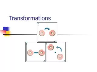
Affine Transformations • Rotation
Affine Transformations • Rotation
Affine Transformations • Rotation
Affine Transformations • Rotation
Affine Transformations • Rotation
Affine Transformations • Uniform Scaling: stretching axis by the same constant factor
Affine Transformations • Nonuniform Scaling: stretching axis by some constant factor, each axis with a different constant
Affine Transformations • Shear: deforms squares into parallelograms
Affine Transformations • Reflection (with respect to a given axis)
Affine Transformations • Line preserving • Maps lines to lines • Translation and rotation preserve lengths and angle • Rigid body transformations • Uniform scaling preserves angles but not lengths • Nonuniform Scaling and shear do not preserve lengths or angles • Importance in graphics is that we need only transform endpoints of line segments and let implementation draw line segment between the transformed endpoints
Affine Transformations • They all preserve affine relationships! R = (1-a)P + aQ T(R) = (1-a)T(P) + aT(Q) • Importance in graphics is that we need only transform endpoints of line segments and let implementation draw line segment between the transformed endpoints • i.e. If we transform endpoints, that is sufficient to obtain linear combinations of transformed endpoints, we do not need to transform every single point R P Q T(Q) T(P)
Pipeline Implementation v T (from application program) frame buffer u T(u) transformation rasterizer T(v) T(v) T(v) v T(u) u T(u) vertices pixels vertices
Notation We will be working with both coordinate-free representations of transformations and representations within a particular frame P,Q, R: points in an affine space u, v, w: vectors in an affine space a, b, g: scalars
Translation • Move (translate, displace) a point to a new location • Displacement determined by a vector d • Three degrees of freedom • P’=P+d P’ d P
How many ways? Although we can move a point to a new location in infinite ways, when we move many points there is usually only one way object translation: every point displaced by same vector
Translation Using Representations Using the homogeneous coordinate representation in some frame P=[ x y z 1]T P’=[x’ y’ z’ 1]T d=[dx dy dz 0]T Hence P’ = P + d or x’=x+dx y’=y+dy z’=z+dz
How to we map P to P’ by matrix multiplication? • P’ = TP • What is T?
How to we map P to P’ by matrix multiplication? • P’ = TP • What is T?
Translation Matrix Hence we can express translation using a 4 x 4 matrix T in homogeneous coordinates P’=TP where T = T(dx, dy, dz) = This form is better for implementation because all affine transformations can be expressed this way and multiple transformations can be concatenated together
Translation • How about vectors under translation transformation? • Vectors are not changed by translation! • Inversion of T? T-1 (dx , dy, dz)= T(-dx, -dy, -dz)
Scaling • Expand or contract along each axis • Performed relative to some fixed point—that is the point remains unchanged after scaling • We will assume that this point is the origin of the standard coordinated frame
Scaling: example in 2D Scale by 2 on x and y axis (2,2) (1,1) (-1,-1) (-2,-2)
Scaling: example in 2D Scale by 2 on x and y axis (4,4) (2,2) (2,2) (1,1)
Scaling • Given scaling factors for each axis, sx,sy,sz, point P is mapped to point P’ as follows • If all scaling factors are equal, that is called uniform scaling x’=sxx y’=syy z’=szz
How to we map P to P’ by matrix multiplication? • P’ = SP • What is matrix S?
How to we map P to P’ by matrix multiplication? • P’ = SP • What is matrix S?
Inverse of Scaling Matrix • S-1(sx, sy, sz) = S(1/sx, 1/sy, 1/sz)
Reflection corresponds to negative scale factors sx = -1 sy = 1 original sx = -1 sy = -1 sx = 1 sy = -1
Rotation (2D) • Consider rotation about the origin by q degrees • Fixed point at the origin • radius stays the same, angle increases by q x’ = r cos (f + q) y’ = r sin (f + q) x = r cos f y = r sin f
Rotation (2D) • Consider rotation about the origin by q degrees • Fixed point at the origin • radius stays the same, angle increases by q x’ = r cos (f + q) y’ = r sin (f + q) x’=r cosfcos q–r sin f sin q y’ = r cos fsin q + r sin fcos q x = r cos f y = r sin f
Rotation (2D) • Consider rotation about the origin by q degrees • Fixed point at the origin • radius stays the same, angle increases by q x’ = r cos (f + q) y’ = r sin (f + q) x’=r cosfcos q–r sin f sin q y’ = r cos fsin q + r sin fcos q x’=x cos q –y sin q y’ = x sin q + y cos q x = r cos f y = r sin f
3D Rotation • In general, rotation happens around an axis and about a fixed point • Assume origin is the fixed point • Consider rotation about z axis • leaves all points with the same z • Equivalent to rotation in 2D in planes of constant z x’=x cos q –y sin q y’ = x sin q + y cos q z’ =z If your thumb is aligned with the axis of rotation, then positive direction is indicated by your fingers: +Q z
3D Rotation Matrix • P’=Rz(q)P Recall: x’=x cos q –y sin q y’ = x sin q + y cos q z’ =z R = Rz(q) =
Rotation about x and y axes • Same argument as for rotation about z axis • For rotation about x axis, x is unchanged • For rotation about y axis, y is unchanged R = Rx(q) = R = Ry(q) =
Fixed Point revisited • The point that remains unchanged through rotation • Example: if the fixed point is origin (center of the square)
Fixed Point revisited • The point that remains unchanged through rotation • Example: if the fixed point is center of the square
Fixed Point revisited • The point that remains unchanged through rotation • Example: if the fixed point is the origin
Inverse Rotation • Although we could compute inverse matrices by general formulas, we can use simple geometric observations • Rotation: R-1(q) = R(-q) • Holds for any rotation matrix • Note that since cos(-q) = cos(q) and sin(-q)=-sin(q) R-1(q) = R T(q)
Concatenation • We can form arbitrary affine transformation matrices by multiplying together rotation, translation, and scaling matrices • Because the same transformation is applied to many vertices, the cost of forming a matrix M=ABCD is not significant compared to the cost of computing Mp for many vertices p • The difficult part is how to form a desired transformation from the specifications in the application
Order of Transformations • Note that matrix on the right is the first applied • Mathematically, the following are equivalent P’ = ABCP = A(B(CP))
Rotation About a Fixed Point other than the Origin (e.g. center of a cube) Translate such that fixed point coincides with origin: T(-pf) Rotate: R(q) Translate fixed point back to its original position: T(pf) Concatenate: M = T(pf) R(q) T(-pf)
General Rotation About the Origin q A rotation by q about an arbitrary axis can be decomposed into the concatenation of rotations about the x, y, and z axes --is a bit complex R(q) = Rz(qz) Ry(qy) Rx(qx) y v qx qy qz are called the Euler angles Note that rotations do not commute We can use rotations in another order but with different angles x z
Instancing • In modeling, we often start with a simple object centered at the origin, oriented with the axis, and at a standard size • We apply an instance transformation to its vertices to Scale Orient Locate
Shear • Helpful to add one more basic transformation • Equivalent to pulling faces in opposite directions
Shear Matrix Consider simple shear along x axis x’ = x + y cot q y’ = y z’ = z H(q) =