Download
1 / 24
250 likes | 455 Vues
MatLab – Palm Chapter 5 Curve Fitting. Class 14.1 Palm Chapter: 5.5-5.7. RAT 14.1. As in INDIVIDUAL you have 1 minute to answer the following question and another 30 seconds to turn it in. Ready? When (day and time) and where is Exam #3? The answer is: Thursday at 6:30 pm,

E N D
MatLab – Palm Chapter 5Curve Fitting Class 14.1 Palm Chapter: 5.5-5.7 ENGR 111A - Fall 2004
RAT 14.1 • As in INDIVIDUAL you have 1 minute to answer the following question and another 30 seconds to turn it in. Ready? • When (day and time) and where is Exam #3? • The answer is: Thursday at 6:30 pm, Bright 124 • Do we have any schedule problems? ENGR 111A - Fall 2004
Learning Objectives • Students should be able to: • Use the Function Discovery (i.e., curve fitting) Techniques • Use Regression Analysis ENGR 111A - Fall 2004
5.5 Function Discovery • Engineers use a few standard functions to represent physical conditions for design purposes. They are: • Linear: y(x) = mx + b • Power: y(x) = bxm • Exponential: y(x) = bemx (Naperian) y(x) = b(10)mx (Briggsian) • The corresponding plot types are explained at the top of p. 299. ENGR 111A - Fall 2004
Steps for Function Discovery • Examine data and theory near the origin; look for zeros and ones for a hint as to type. • Plot using rectilinear scales; if it is a straight line, it’s linear. Otherwise: • y(0) = 0 try power function • Otherwise, try exponential function • If power function, log-log is a straight line. • If exponential, semi-log is a straight line. ENGR 111A - Fall 2004
Example Function Calls • polyfit( ) will provide the slope and y-intercept of the BEST fit line if a line function is specified. • Linear: polyfit(x, y, 1) • Power: polyfit(log10(x),log10(y),1) • Exponential: polyfit(x,log10(y),1); Briggsian polyfit(x,log(y),1); Naperian Note: the use of log10( ) or log( ) to transform the data to a linear dataset. ENGR 111A - Fall 2004
Example 5.5-1:Cantilever Beam Deflection • First, input the data table on page 304. • Next, plot deflection versus force (use data symbols or a line?) • Then, add axes and labels. • Use polyfit() to fit a line. • Hold the plot and add the fitted line to your graph. ENGR 111A - Fall 2004
Solution ENGR 111A - Fall 2004
Straight Line Plots ENGR 111A - Fall 2004
Why do these plot as lines? Exponential function: y = bemx Take the Naperian logarithm of both sides: ln(y) = ln(bemx) ln(y) = ln(b) + mx(ln(e)) ln(y) = ln(b) + mx Thus, if the x value is plotted on a linear scale and the y value on a log scale, it is a straight line with a slope of m and y-intercept of ln(b). ENGR 111A - Fall 2004
Why do these plot as lines? Exponential function: y = b10mx Take the Briggsian logarithm of both sides: log(y) = log(b10mx) log(y) = log(b) + mx(log(10)) log(y) = log(b) + mx Thus, if the x value is plotted on a linear scale and the y value on a log scale, it is a straight line. (Same as Naperian.) ENGR 111A - Fall 2004
Why do these plot as lines? Power function: y = bxm Take the Briggsian logarithm of both sides: log(y) = log(bxm) log(y) = log(b) + log(xm) log(y) = log(b) + mlog(x) Thus, if the x and y values are plotted on a on a log scale, it is a straight line. (Same can be done with Naperian log.) ENGR 111A - Fall 2004
In-class Assignment 14.1.1 Given: x=[1 2 3 4 5 6 7 8 9 10]; y1=[3 5 7 8 10 14 15 17 20 21]; y2=[3 8 16 24 34 44 56 68 81 95]; y3=[8 11 15 20 27 36 49 66 89 121]; • Use MATLAB to plot x vs each of the y data sets. • Chose the best coordinate system for the data. • Be ready to explain why the system you chose is the best one. ENGR 111A - Fall 2004
Solution ENGR 111A - Fall 2004
Be Careful • What value does the first tick mark after 100 represent? What about the tick mark after 101 or 102? • Where is zero on a log scale? Or -25? • See pages 282 and 284 of Palm for more special characteristics of logarithmic plots. ENGR 111A - Fall 2004
How to use polyfit command. • Linear: pl = polyfit(x, y, 1) • m = pl(1); b = pl(2) of BEST FIT line. • Power: pp = polyfit(log10(x),log10(y),1) • m = pp(1); b = 10^pp(2) of BEST FIT line. • Exponential: pe = polyfit(x,log10(y),1) • m = pe(1); b = 10^pe(2), best fit line using Briggsian base. OR pe = polyfit(x,log(y),1) • m = pe(1); b = exp(pe(2)), best fit line using Naperian base. ENGR 111A - Fall 2004
In-class Assignment 14.1.2 • Determine the equation of the best-fit line for each of the data sets in In-class Assignment 14.1.1 • Hint: use the result from ICA 14.1.1 and the polyfit( ) function in MatLab. • Plot the fitted lines in the figure. ENGR 111A - Fall 2004
Solution ENGR 111A - Fall 2004
5.6 Regression Analysis • Involves a dependent variable (y) as a function of an independent variable (x), generally: y = mx + b • We use a “best fit” line through the data as an approximation to establish the values of: m = slope and b = y-axis intercept. • We either “eye ball” a line with a straight-edge or use the method of least squares to find these values. ENGR 111A - Fall 2004
Curve Fits by Least Squares • Use Linear Regression unless you know that the data follows a different pattern: like n-degree polynomials, multiple linear, log-log, etc. • We will explore 1st (linear), … 4th order fits. • Cubic splines (piecewise, cubic) are a recently developed mathematical technique that closely follows the “ship’s” curves and analogue spline curves used in design offices for centuries for airplane and ship building. • Curve fitting is a common practice used my engineers. ENGR 111A - Fall 2004
T5.6-1 • Solve problem T5.6-1 on page 318. • Notice that the fit looks better the higher the order – you can make it go through the points. • Use your fitted curves to estimate y at x = 10. Which order polynomial do you trust more out at x = 10? Why? ENGR 111A - Fall 2004
Solution ENGR 111A - Fall 2004
Solution ENGR 111A - Fall 2004
Assignment 14.1 • Prepare for Exam #3. • Group Projects are due at Exam #3(parts 1 through 3 required; parts 4 and 5 as extra credit) ENGR 111A - Fall 2004