Matlab Training Session 11: Nonlinear Curve Fitting
530 likes | 971 Vues
Matlab Training Session 11: Nonlinear Curve Fitting. Course Website: http://www.queensu.ca/neurosci/Matlab Training Sessions.htm. Course Outline Term 1 Introduction to Matlab and its Interface Fundamentals (Operators) Fundamentals (Flow) Importing Data Functions and M-Files

Matlab Training Session 11: Nonlinear Curve Fitting
E N D
Presentation Transcript
Matlab Training Session 11:Nonlinear Curve Fitting • Course Website: • http://www.queensu.ca/neurosci/Matlab Training Sessions.htm
Course Outline Term 1 • Introduction to Matlab and its Interface • Fundamentals (Operators) • Fundamentals (Flow) • Importing Data • Functions and M-Files • Plotting (2D and 3D) • Plotting (2D and 3D) • Statistical Tools in Matlab Term 2 9. Term 1 review 10. Loading Binary Data 11. Nonlinear Curve Fitting 12. Statistical Tools in Matlab II
Week 11 Lecture Outline Nonlinear Curve Fitting • Linear Curve Fitting Review • Calculating Linear Regressions • Least Squares vs Robust Fit • Figure Window Curve Fitting Interface • Curve Fitting Toolbox • Curve Fitting Strategies • Calculating Goodness of Fit
Week 11 Lecture Outline Required Toolboxes: • Statistics Toolbox • Curve Fitting Toolbox • Spline Toolbox
Week 11 Lecture Outline Purpose of Curve Fitting: • Curve fitting matches mathematical models to data • Is a powerful tool if it can be used to make accurate predictions
Week 11 Lecture Outline Nonlinear Curve Fitting Part A: Linear Curve Fitting Review
Curve Fitting • Plotting a line of best fit in Matlab can be performed using either a traditional least squares fit or a robust fitting method. • Robust Vs Least Squares Demo (robustdemo) 12 10 8 6 Least squares 4 Robust 2 0 -2 1 2 3 4 5 6 7 8 9 10
Curve Fitting • A least squares linear fit minimizes the square of the distance between every data point and the line of best fit polyfit(X,Y,N) finds the coefficients of a polynomial P(X) of degree N that fits the data Uses least-square minimization N = 1 (linear fit) [P] = polyfit(X,Y,N) returns P, a matrix containing the slope and the x intercept for a linear fit [Y] = polyval(P,X) calculates the Y values for every X point on the line of best fit
Curve Fitting • Example: • Draw a line of best fit using least squares approximation for the data in exercise 2 [var1, var2] = textread('testdata2.txt','%f%f','headerlines',1) P = polyfit(var1,var2,1); Y = polyval(P,var1); close all figure(1) hold on plot(var1,var2,'ro') plot(var1,Y)
Curve Fitting • A least squares linear fit minimizes the square of the distance between every data point and the line of best fit • A robust fit is less effected by small numbers of outliers • P = robustfit(X,Y) returns the vector B of the y intercept and slope, obtained by performing robust linear fit • ‘robustdemo’ gives a good graphical example comparing robust and least squares line fitting
Curve Fitting Example: • Draw a line of best fit using robust fit approximation for the data in exercise 2 [var1, var2] = textread('testdata2.txt','%f%f','headerlines',1) P = robustfit(var1,var2,1); Y = polyval([P(2),P(1)],var1); close all figure(1) hold on plot(var1,var2,'ro') plot(var1,Y)
Higher Order Curve Fitting Method 1 • Polyfit can be used to calculate any polynomial fitting function of the form: • y = polyval(p,x) returns the value of a polynomial of degree n evaluated at x. The input argument p is a vector of length n+1 whose elements are the coefficients in descending powers of the polynomial to be evaluated. • x can be a matrix or a vector. In either case, polyval evaluates p at each element of x.
Curve Fitting Example: • Calculate a polynomial fit of order 2, 3, and 4 for the data in the previous example
Curve Fitting Example • 2nd Order Polynomial Fit: %read data [var1, var2] = textread(‘week8_testdata2.txt','%f%f','headerlines',1) % Calculate 2nd order polynomial fit P2 = polyfit(var1,var2,2); Y2 = polyval(P2,var1); %Plot fit close all figure(1) hold on plot(var1,var2,'ro') [sortedvar1, sortind] = sort(var1) plot(sortedvar1,Y2(sortind),'b*-')
Curve Fitting Example • Add 3rd Order Polynomial Fit: % Calculate 3rd order polynomial fit P3 = polyfit(var1,var2,3); Y3 = polyval(P3,var1); %Add fit to figure figure(1) plot(sortedvar1,Y3(sortind),’g*-')
2nd Order Polynomial Fit: 3rd Order Polynomial Fit:
Curve Fitting Example • Add 4th Order Polynomial Fit: % Calculate 4th order polynomial fit P4 = polyfit(var1,var2,4); Y4 = polyval(P4,var1); %Add fit to figure figure(1) plot(sortedvar1,Y4(sortind),’k*-')
2nd Order Polynomial Fit: 3rd Order Polynomial Fit: 4th Order Polynomial Fit:
Assessing Goodness of Fit • The tough part of polynomial regression is knowing that the "fit" is a good one. • Determining the quality of the fit requires experience, a sense of balance and some statistical summaries.
Assessing Goodness of Fit • One common goodness of fit involves a least-squares approximation. This describes the distance of the entire set of data points from the fitted curve. The normalization of the residual errorminimizing the square of the sum of squares of all residual errors. • The coefficient of determination (also referred to as the R2 value) for the fit indicates the percent of the variation in the data that is explained by the model.
Assessing Goodness of Fit • This coefficient can be computed via the commands: ypred = polyval(coeff,x); % predictions dev = y - mean(y); % deviations - measure of spread SST = sum(dev.^2); % total variation to be accounted for resid = y - ypred; % residuals - measure of mismatch SSE = sum(resid.^2); % variation NOT accounted for normr = sqrt(SSE) % the 2-norm of the vector of the residuals for the fit Rsq = 1 - SSE/SST; % R2 Error (percent of error explained) • The closer that Rsq is to 1, the more completely the fitted model "explains" the data.
Assessing Goodness of Fit Example: • Calculate the R2 error and Norm of the residual error for a 2nd order polynomial fit for the data in the previous example
Assessing Goodness of Fit Example Solution % recall var1 contains x values and var2 contains y values of data points ypred = polyval(P2,var1); dev = var2 - mean(2); SST = sum(dev.^2); resid = var2 - ypred; SSE = sum(resid.^2); normr = sqrt(SSE); % residual norm Rsq = 1 - SSE/SST; % R2 Error Normr = 5.7436 Rsq = 0.8533 • The residual norm and R2 error indicate goodness of fit 2nd Order Polynomial Fit:
Limitations of Polyfit • Only finds a least squares best polynomial function fit • Cannot be used to interpolate curves or fit other standard functions • Requires several lines of code and the polyval() function
Higher Order Curve Fitting Method 2 • Curve Fitting Tools can be accessed directly from the figure window: • To access curve fitting directly from the figure window, select ‘basic fitting’ from the ‘tools’ pulldown menu in the figure window. • This is a quick and easy method to calculate and visualize a variety of higher order functions including interpolation
Higher Order Curve Fitting Method 2 • Plot data from previous exercise • Try a variety of curve fittings
Higher Order Curve Fitting Caution: • Higher order polynomial fits should only be used when a large number of data points are available • Higher order polynomial fitting functions may fit more the data more accurately but may not yield an interpretable model
Higher Order Curve Fitting Method 2 Curve Fitting from Figure Window Advantages: • Quick and easy to plot fits from existing data Easy accessibility of: • Function Coefficients • Fitting Equations • Residual errors • The value of fitting function at any value of x
Higher Order Curve Fitting Method 3 • Curve Fitting Toolbox • The curve fitting toolbox is accessible by the ‘cftool’ command • Very powerful tool for data smoothing, curve fitting, and applying and evaluating mathematical models to data points
Curve Fitting Toolbox 1. Loading Data Sets • Before you can import data into the Curve Fitting Tool, the data variables must exist in the MATLAB workspace. • You can import data into the Curve Fitting Tool with the Data GUI. You open this GUI by clicking the Data button on the Curve Fitting Tool. • The Data Sets pane allows you to: Import predictor (X) data, response (Y) data, and weights. • If you do not import weights, then they are assumed to be 1 for all data points. • Specify the name of the data set. • Preview the data. • Click the Create data set button to complete the data import process.
Curve Fitting Toolbox 2. Smoothing Data Points • If your data is noisy, you might need to apply a smoothing algorithm to expose its features, and to provide a reasonable starting approach for parametric fitting.
Curve Fitting Toolbox 2. Smoothing Data Points • If your data is noisy, you might need to apply a smoothing algorithm to expose its features, and to provide a reasonable starting approach for parametric fitting. The two basic assumptions that underlie smoothing are: 1. The relationship between the response data and the predictor data is smooth. 2. The smoothing process results in a smoothed value that is a better estimate of the original value because the noise has been reduced.
Curve Fitting Toolbox 2. Smoothing Data Points • The Curve Fitting Toolbox supports these smoothing methods: Moving Average Filtering: Lowpass filter that takes the average of neighboring data points. Lowess and Loess: Locally weighted scatter plot smooth. These methods use linear least squares fitting, and a first-degree polynomial (lowess) or a second-degree polynomial (loess). Robust lowess and loess methods that are resistant to outliers are also available. Savitzky-Golay Filtering: A generalized moving average where you derive the filter coefficients by performing an unweighted linear least squares fit using a polynomial of the specified degree.
Curve Fitting Toolbox • Smoothing Method and Parameters • Span: The number of data points used to compute each smoothed value. • For the moving average and Savitzky-Golay methods, the span must be odd. For all locally weighted smoothing methods, if the span is less than 1, it is interpreted as the percentage of the total number of data points. • Degree: The degree of the polynomial used in the Savitzky-Golay method. The degree must be smaller than the span.
Curve Fitting Toolbox Excluding Data Points • It may be necessary to remove outlier points from a data set before attempting a curve fit • Typically, data points are excluded so that subsequent fits are not adversely affected. • Can help improve a mathematical model’s predictability
Curve Fitting Toolbox Excluding Data Points The Curve Fitting Toolbox provides two methods to exclude data: • Marking Outliers: Outliers are defined as individual data points that you exclude because they are inconsistent with the statistical nature of the bulk of the data. • Sectioning: Sectioning excludes a window of response or predictor data. For example, if many data points in a data set are corrupted by large systematic errors, you might want to section them out of the fit. • For each of these methods, you must create an exclusion rule, which captures the range, domain, or index of the data points to be excluded.
Curve Fitting Toolbox Plotting Fitting Curves • You fit data with the Fitting GUI. You open this GUI by clicking the Fitting button on the Curve Fitting Tool.
Curve Fitting Toolbox Plotting Fitting Curves The Fit Editor allows you to: • Specify the fit name, the current data set, and the exclusion rule. • Explore various fits to the current data set using a library or custom equation, a smoothing spline, or an interpolant. • Override the default fit options such as the coefficient starting values. • Compare fit results including the fitted coefficients and goodness of fit statistics.
Curve Fitting Toolbox Plotting Fitting Curves The Table of Fits allows you to: • Keep track of all the fits and their data sets for the current session. • Display a summary of the fit results. • Save or delete the fit results.
Curve Fitting Toolbox Analyzing Fits • You can evaluate (interpolate or extrapolate), differentiate, or integrate a fit over a specified data range with the Analysis GUI. You open this GUI by clicking the Analysis button on the Curve Fitting Tool.
Curve Fitting Toolbox Analyzing Fits To Test your Model’s Predictions: • Enter the appropriate MATLAB vector in the Analyze at Xi field. • Select the Evaluate fit at Xi check box. • Select the Plot results and Plot data set check boxes. • Click the Apply button. • The numerical extrapolation results are displayed
Curve Fitting Toolbox Saving Your Work • You can save one or more fits and the associated fit results as variables to the MATLAB workspace. • You can then use this saved information for documentation purposes, or to extend your data exploration and analysis. • In addition to saving your work to MATLAB workspace variables, you can: 1. Save the session 2. Generate an M-file
Curve Fitting Toolbox Saving Your Work Generating an M-file: • You may want to generate an M-file so that you can continue data exploration and analysis from the MATLAB command line. • You can run the M-file without modification to recreate the fits and results that you created with the Curve Fitting Tool, or you can edit and modify the file as needed
Curve Fitting Toolbox Saving Your Work Generating an M-file: The M-file captures: • All data set variable names, associated fits, and residuals • Fit options such as whether the data should be normalized, the fit starting points, and the fitting method • You can recreate the saved fits in a new figure window by typing the name of the M-file at the MATLAB command line. • Note that you must provide the appropriate data variables as inputs to the M-file. These variables are given in the M-file help.
Curve Fitting Toolbox Exercise 1. Load the data file ‘week8_testdata2.txt’ from week 8 2. Use the curve fitting toolbox smooth the data using a 5 point moving average 3. Exclude all points with y values less then -1 4. Fit a 4th order polynomial through the smoothed data points 5. Generate an m-file that can be used to re-calculate the fitted curve
Getting Help • Help and Documentation • Digital • Accessible Help from the Matlab Start Menu • Updated online help from the Matlab Mathworks website: • http://www.mathworks.com/access/helpdesk/help/techdoc/matlab.html • Matlab command prompt function lookup • Built in Demo’s • Websites • Hard Copy • Books, Guides, Reference • The Student Edition of Matlab pub. Mathworks Inc.