Download

1 / 92
920 likes | 1.03k Vues
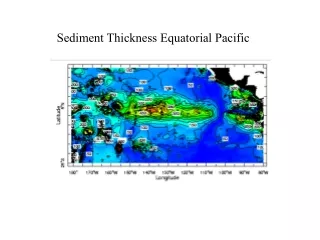
Explore improvements in modeling Equatorial Pacific cold tongue region's impact on climate dynamics, cloud cover, and oceanic productivity. Addressing biases in OGCM output.

E N D
In revisions at the Journal of Physical Oceanography Improvements to the Equatorial Pacific Cold Tongue Region in an OGCM Possible Implications for the NCEP GODAS / CFS Kristopher B. Karnauskas, Raghu Murtugudde, Antonio J. Busalacchi University of Maryland College Park, Md., USA Photo of Isla Isabela NOAA R/V Ka’imimoana 2 May 2005 NOAA NCEP/EMC 6/20/06
In revisions at the Journal of Physical Oceanography Improvements to the Equatorial Pacific Cold Tongue Region in an OGCM Possible Implications for the NCEP GODAS / CFS “The currents of the sea are rapid and sweep across the [Galapagos] archipelago, and the gales of wind are extraordinarily rare…” “Considering that these islands are placed directly under the equator, the climate is far from being excessively hot; this seems chiefly caused by the singularly low temperatures of the surrounding water…” - British Naturalist Charles Darwin in 1859 and 1839
Introduction: The Pacific cold tongue is… TMI SST Annual Mean (1998-2005) • A zonal band of cold SST along the equator in the east-central Pacific. • The result of coastal upwelling and Ekman divergence, a true coupled air- sea interaction process. • Linked to tropical cloud and precipitation patterns, ocean biological productivity and carbon cycling.
Introduction: The Pacific cold tongue is… Mean CMAP Precipitation • Linked to tropical cloud and precipitation patterns, ocean biological productivity and carbon cycling.
Introduction: The Pacific cold tongue is… Mean SeaWiFS Surface Chlorophyll-a • Linked to tropical cloud and precipitation patterns, ocean biological productivity and carbon cycling.
Introduction: The Pacific cold tongue is… Mean Ocean-Atmosphere Carbon Flux (Takahashi et al., 1999) • Linked to tropical cloud and precipitation patterns, ocean biological productivity and carbon cycling. • Linked to tropical cloud and precipitation patterns, ocean biological productivity and carbon cycling. • Where ENSO events produce large SST anomalies.
Introduction: The Pacific cold tongue is… TMI SST: December 1997 • Linked to tropical cloud and precipitation patterns, ocean biological productivity and carbon cycling. • Linked to tropical cloud and precipitation patterns, ocean biological productivity and carbon cycling. • Where ENSO events produce large SST anomalies.
Introduction: Tropical cold bias (Vecchi et al., 2005) • Problem: most OGCMs produce a cold tongue that is too cold and extends too far west… • Problem: most OGCMs produce a cold tongue that is too cold and extends too far west… • Presents obstacles for coupled GCMs to produce realistic tropical cloud and precipitation patterns… one potential culprit in the “double ITCZ” problem. • A relevant theme in ongoing and upcoming research programs, e.g. Pacific Upwelling and Mixing Physics (PUMP). • Modeling studies aimed at diagnosing the cold bias have focused on the surface energy budget (Kiehl, 1997), atmospheric feedbacks (Gordon et al., 2000; Sun et al., 2003), biological attenuation of shortwave radiation (Murtugudde et al., 2002, Marzeion et al., 2005) and otherwise coupled air-sea interactions (Luo et al., 2004). • These studies represent progress, but the cold bias remains a serious problem. There also remain problems with the EUC and SEC.
Introduction: Current ocean modeling Image courtesy Dave Behringer and Yan Xue, http://www.nws.noaa.gov/ost/climate/STIP/GODAS.htm The GODAS, a part of the CFS, is based on the MOM3 OGCM. Currently 1° x 1° with 1/3° meridional within 10° of the equator. 1982-2004
Introduction: Current ocean modeling The GODAS, a part of the CFS, is based on the MOM3 OGCM. Currently 1° x 1° with 1/3° meridional within 10° of the equator. 1982-2004
Introduction: Current ocean modeling The GODAS, a part of the CFS, is based on the MOM3 OGCM. Currently 1° x 1° with 1/3° meridional within 10° of the equator.
Introduction: Current ocean modeling • What has not been considered explicitly are the effects of horizontal resolution and the inclusion of the Galapagos Islands in the models. • The Galapagos Islands are directly on the equator, in the midst of the cold tongue… and in a very critical place in terms of surface fluxes and subsurface currents. • Current operational ocean modeling at NOAA NCEP does not include the Galapagos Islands. GODAS horizontal resolution is arguably sufficient to represent them.
Introduction: Current ocean modeling Galapagos topography in the GODAS / CFS Thanks to Dave Behringer (NCEP/EMC) for kindly providing this figure.
Introduction: Current ocean modeling • What has not been considered explicitly are the effects of horizontal resolution and the inclusion of the Galapagos Islands in the models. • The Galapagos Islands are directly on the equator, in the midst of the cold tongue… and in a very critical place in terms of surface fluxes and subsurface currents. • Current operational ocean modeling at NOAA NCEP does not include the Galapagos Islands. GODAS horizontal resolution is arguably sufficient to resolve them. • Effects of the Galapagos Islands in an OGCM (MOM3) were looked at by Eden & Timmerman (2004) but there are some concerns about how that was done. Also, ET-04 focused on very local-scale effects (TIWs and island upwelling). However, ET-04 provides useful comparison with our study.
Experimental philosophy Kraus-Turner (1967) type mixed layer model Price et al. (1986) dynamical instability model Chen et al. (1994) HYBRID... • Gent & Cane (1989) OGCM coupled to an atmospheric mixed layer (just surface fluxes; Murtugudde et al., 1996) and hybrid vertical mixing scheme (Chen et al., 1994a). This model has been extensively tested and used successfully in the tropical Pacific (e.g. Kessler et al., 1998; Chen et al., 1994a,b and many others). • Nicely captures the 3 major physical processes of vertical entrainment-mixing: • Mixed layer entrainment-detrainment (related to atmospheric forcing) • Shear flow instability (Richardson-dependent) • Free convection in thermocline (instant adjustment)
Experimental philosophy • Gent & Cane (1989) OGCM coupled to an atmospheric mixed layer (just surface fluxes; Murtugudde et al., 1996) and hybrid vertical mixing scheme (Chen et al., 1994a). This model has been extensively tested and used successfully in the tropical Pacific (e.g. Kessler et al., 1998; Chen et al., 1994a,b and many others). • Some modifications: higher-order Shapiro filter (8th), shorter time-step (30 min.), and grid-stretching in the zonal direction as opposed to just y-stretching…
Experimental philosophy • A total of 4 one-year climatology simulations… after being spun up onto each grid independently (60 years plus “spin-overs”). • Coarse Uniform zonal resolution, no Galapagos • Coarse+G Uniform zonal resolution, with Galapagos • FineHigher (stretched) zonal resolution, no Galapagos • Fine+GHigher (stretched) zonal resolution, with Galapagos • Forcing was climatological ECMWF winds, Xie & Arkin precipitation, ISCCP clouds, and ERBE shortwave. • Validation data used were Reynolds, TMI and TAO. XRES: uniform 3/4, YRES: 1/3° stretching to 1° XRES: 1/4° stretching to 1°, YRES: 1/4° stretching to 1°
Experimental philosophy 0° 1°S
Experimental philosophy Coarse Fine
Results: Comparing annual mean SST Coarse Coarse+G Fine Fine+G TMI Contour Interval: 1°C Shaded: SST < 23°C Bold contour: 26°C
Results: Comparing annual mean SST Coarse Coarse+G Fine Fine+G TMI Contour Interval: 1°C Shaded: SST < 23°C Bold contour: 26°C
Results: Comparing annual mean SST Coarse Coarse+G Fine Fine+G TMI Contour Interval: 1°C Shaded: SST < 23°C Bold contour: 26°C
Results: Comparing annual mean SST Coarse Coarse+G Fine Fine+G TMI Contour Interval: 1°C Shaded: SST < 23°C Bold contour: 26°C
Results: SST seasonal cycle A cold tongue index (1998-2005 Annual Mean TMI SST)
Results: Seasonal SST fields Mar-Apr-May Sep-Oct-Nov Coarse Coarse+G Fine Fine+G TMI Contour Interval: 1°C Shaded: SST < 24°C Bold contour: 27°C Contour Interval: 1°C Shaded: SST < 22°C Bold contour: 26°C
Results: Seasonal SST fields Mar-Apr-May Sep-Oct-Nov Coarse Coarse+G Fine Fine+G TMI Contour Interval: 1°C Shaded: SST < 24°C Bold contour: 27°C Contour Interval: 1°C Shaded: SST < 22°C Bold contour: 26°C
Results: Seasonal SST fields Mar-Apr-May Sep-Oct-Nov Coarse Coarse+G Fine Fine+G TMI Contour Interval: 1°C Shaded: SST < 24°C Bold contour: 27°C Contour Interval: 1°C Shaded: SST < 22°C Bold contour: 26°C
Results: Seasonal SST fields Mar-Apr-May Sep-Oct-Nov Coarse Coarse+G Fine Fine+G TMI Contour Interval: 1°C Shaded: SST < 24°C Bold contour: 27°C Contour Interval: 1°C Shaded: SST < 22°C Bold contour: 26°C
Results: SST seasonal cycle 2° x 2° box indices (1998-2005 Annual Mean TMI SST)
Results: SST seasonal cycle Coarse Resolution
Results: SST seasonal cycle High Resolution
Results The EUC
Results: Zonal Currents and Temperature GODAS TAO Clim. Adapted from Large, et al. (2001) Coarse Fine Coarse+G Fine+G (Sep-Oct-Nov)
Results: Zonal currents at 100m * This is our model “off the shelf.” No tuning.
Results: Zonal currents in the RA6 & GODAS Fine Fine+G Mean Zonal Currents RMSE w.r.t. TAO (Adapted from Behringer and Xue, 2004) (Annual Mean)
Results: Termination of the EUC Fine Fine+G
Results: Termination of the EUC Fine Fine+G
Results: (Non-)Termination of the EUC (Eden & Timmerman, 2004)
Results: The EUC from all angles 0m 10m 20m 30m 40m 50m 60m 70m 80m 90m 100m 110m 120m 130m 140m 150m 160m 170m 180m 190m 200m Fine Fine+G
Results: The EUC from all angles 0m 10m 20m 30m 40m 50m 60m 70m 80m 90m 100m 110m 120m 130m 140m 150m 160m 170m 180m 190m 200m Fine Fine+G
Results: The EUC from all angles 0m 10m 20m 30m 40m 50m 60m 70m 80m 90m 100m 110m 120m 130m 140m 150m 160m 170m 180m 190m 200m Fine Fine+G
Results: The EUC from all angles 0m 10m 20m 30m 40m 50m 60m 70m 80m 90m 100m 110m 120m 130m 140m 150m 160m 170m 180m 190m 200m Fine Fine+G
Results: The EUC from all angles 0m 10m 20m 30m 40m 50m 60m 70m 80m 90m 100m 110m 120m 130m 140m 150m 160m 170m 180m 190m 200m Fine Fine+G
Results: The EUC from all angles 0m 10m 20m 30m 40m 50m 60m 70m 80m 90m 100m 110m 120m 130m 140m 150m 160m 170m 180m 190m 200m Fine Fine+G
Results: The EUC from all angles 0m 10m 20m 30m 40m 50m 60m 70m 80m 90m 100m 110m 120m 130m 140m 150m 160m 170m 180m 190m 200m Fine Fine+G
Results: The EUC from all angles 0m 10m 20m 30m 40m 50m 60m 70m 80m 90m 100m 110m 120m 130m 140m 150m 160m 170m 180m 190m 200m Fine Fine+G
Results: The EUC from all angles 0m 10m 20m 30m 40m 50m 60m 70m 80m 90m 100m 110m 120m 130m 140m 150m 160m 170m 180m 190m 200m Fine Fine+G