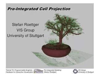
Pre-Integrated Cell Projection
Pre-Integrated Cell Projection. Stefan Roettger VIS Group University of Stuttgart. Pre-Integrated Cell Projection. Stefan Roettger VIS Group University of Stuttgart. Unstructured Volume Rendering. Given an irregular volumetric mesh How can the volume be rendered accurately?

Pre-Integrated Cell Projection
E N D
Presentation Transcript
Pre-Integrated Cell Projection Stefan Roettger VIS Group University of Stuttgart Pre-Integrated Cell Projection Stefan Roettger VIS Group University of Stuttgart
Unstructured Volume Rendering • Given an irregular volumetric mesh • How can the volume be rendered accurately? • Obvious: Resampling to regular grid • Too heavy: Ray tracing • Ray casting • Sweep plane algorithms • Cell projection
Resampling to Regular Grid • Hardware-accelerated: Westermann et al. [1] • Use graphics hardware to compute the intersection of a set of tetrahedra with a slice plane. • Comparison with software: Weiler et al. [2] • Comparison hardware/software approach. • It turns out that software is not significantly slower than a PC hardware based resampling approach.
Ray Tracing • Basic Algorithm: • Shoot rays through the volume and integrate the ray integral at each cell intersection in a back to front fashion taking scattering into account. • Pros: • Physically based accurate method • Cons: • Dependend on view port resolution • Very slow, but can be parallelized
Ray Casting • Basic algorithm: • Shoot rays through the volume in a front to back fashion and accumulate the ray integral neglecting scattering processes inside the media. • Pros: • Faster because of simplified physical model • Early ray termination and space leaping • Runs on every platform • Cons: • Dependend on view port size
Sweep Plane Algorithms • Basic algorithm: • Use a sweep plane to process the cells in a back to front fashion and compose the cells. • E.g. ZSWEEP (Farias et al. [3]) • Pros: • Runs on every platform • Easy to parallelize • Cons: • Dependent on view port size
Splatting • Basic algorithm: • Approximate each cell with a volumetric blob and compose the footprints in a back to front fashion. • Pros: • Good performance, since footprints can be rendered by the graphics hardware. • Object order method • Cons: • Footprint is only an approximation blurry look
Cell Projection • „Accurate Splatting“ • Basic algorithm: • Sort the cells in a back to front fashion and compose the geometric projections of the cells. • Pros: • Hardware-accelerated / Accurate composing • Object order method • Cons: • Projection of non-tetrahedral cells is difficult • Topological sort needed
The PT Algorithm of Shirley and Tuchman • We distinguish between two different non-degenerate classes of projected tetrahedra: "thick vertex" use triangle fanning to render decomposed triangles around thick vertex according to [4]
Topological Sorting • Numerical (Wittenbrink et al. [5]) • fast but incorrect • MPVO (Williams et al. [6]) • sorts convex polyhedra by processing the hidden relationship via a priority queue • XMPVO (Silva et al. [7]) • BSP-XMPVO (Comba et al. [8]) • constructs external dependencies via BSP-tree • MPVOC (Kraus et al. [9]) • extension of MPVO which can handle cycles
Optical Model of Williams et al. • "Volume Density Optical Model" (Williams et al. [10]) • Emission and absorption along each ray segment depends on the scalar function f(x,y,z). • The scalar optical density and chromaticity is defined by the transfer functions r(f(x,y,z)) and k(f(x,y,z)).
Approximation of Stein et al. • Approximation of the ray integral by Stein et al. [11] for linear transfer function r and a constant transfer function k: • a=1-exp(-lt) • l=length of ray segment • t=average optical density • t=(r(Sf)+r(Sb))/2
Approximation of Stein et al. • Put alpha(l,t) into 2D texture and assign (l,t) as texture coordinates to projected vertices. • Linear interpolation of texture coordinates yields exponentially interpolated opacities.
Approximation of Stein et al. • Pros: • Hardware-accelerated • 2D texture mapping only • Equivalent to 1D dependent texture today • Cons: • Restricted application of transfer functions • Transfer functions cannot be taken into account inside the tetrahadra
Pre-Integrated Cell Projection • Observation: The ray integral depends only on Sf,Sb, and l. • Pre-compute the three-dimensional ray integral by numerical integration and store it in a 3D texture. • Assign appropriate 3D texture coords (Sf,Sb,l) to each projected vertex and use 3D texture mapping to perform per-pixel exact compositing. • This approach is known as Pre-Integration [12]
Numerical Pre-Integration • The Ray Integral:
Numerical Pre-Integration iterate over l iterate over Sb iterate over Sf chromaticity C0=0 transparency T0=1 iterate over #steps (i=0...n-1) S=(1-i/(n-1))Sb+i/(n-1)Sf compute emission=k(S)*l/(n-1) compute absorption=exp(-r(S)*l/(n-1)) Ci+1=Ci*absorption+emission Ti+1=Ti*absorption Tex3D(Sf,Sb,l)=(Cn-1,1-Tn-1)
Pre-Integration Example Simple spherical distance volume rendered with piecewise transparent transfer function. The integrated chromaticity is shown below.
Pre-Integrated Cell Projection • Pros: • Arbitrary transfer functions can be used • Accuracy only limited by the size of the pre-intgration table • Per-pixel exact rendering • Unshaded isosurfaces with Dirac Delta • Cons: • 3D textures not available everywhere • Memory consumption of 3D textures
Rendering of Unshaded Isosurfaces • Render Isosurfaces with the Dirac Delta as the transfer function -> unshaded isosurfaces Ray integral of three Dirac Deltas with different colors
Shaded Isosurfaces • Two passes required for shaded isosurfaces • First pass: Render lit back faces with left texture. • Second pass: Render lit front faces with right texture which contains the correct interpolation factor.
Shaded Isosurfaces • Multiple shaded isosurfaces extracted simultaneously
Mixing with Shaded Isosurfaces • Additional third pass for mixed volume and isosurface rendering. • Pre-Integration is stopped if an isosurface is encountered to ensure correct mixing.
Mixing with Shaded Isosurfaces • Multiple shaded isosurfaces mixed with the pre-integrated volume • Note that the volume is cut correctly at the isosurfaces.
Mixing with Shaded Isosurfaces A Bonsai Tree
Reparametrization of the 3D Ray Integral • Observation: Rasterized pixels of a tetrahedron lie on a plane in texture coordinate space [13].
Reparametrization of the 3D Ray Integral 8 Slices of a 64^3 3D texture Corresponding tiled 2D texture TF
Separation of the 3D Texture • Use the pixel shader on the PC platform to separate the three-dimensional ray integral [14]. • Opacity can be separated easily by means of 1D dependent texture lookup for exp() function. linear opacity exponential opacity
Separation of the 3D Texture • Chromaticity cannot be separated, it can only be approximated: • Construct quadratic polynomial in l through every pair of Sf and Sb and store the coefficients for RGB in multiple 2D texture maps. • Reconstruct the original color in the pixel shader. n=1 n=2
Separation of the 3D Texture • Pros: • High resolutions possible since only three 2D plus one 1D textures are kept in graphics memory for n=2 • Faster texturing since 3D textures are slow
Hardware-Accelerated Pre-Integration • Accelerate the numerical integration using graphics hardware to maintain interactive updates of the pre-intgration table [13]. • Prerequisite for comfortable exploration of unstructured data sets • Basic Idea: Put the transfer function in a 1D texture and compute one slice of the 3D texture for l=const in parallel.
Hardware-Accelerated Pre-Integration • Pros: • Numerical integration takes >1min for a 512x512x64 pre-integration table. • With hardware acceleration update rates of <1s are achieved easily. • Cons: • Quantization artifacts but with pixel shader 14 bits [14] - *8 =
Application to Cloud Rendering • View-dependent simplification of regular volume • Screen space error of the simplification is bounded by a user definable threshold. • Octree hierarchy • is decomposed • into tetrahedra
Application to Cloud Rendering • Clouds generated with 3D Perlin noise • Ground fog displayed by stacking prisms onto each triangle that is generated by the C-LOD terrain renderer avg. 25 fps.
Bibliography (1) • [1] R. Westermann. The Rendering of Unstructured Grids Revisited. Proc. IEEE VisSym '01. 2001. • [2] M. Weiler and Th. Ertl. Hardware-Software-Balanced Resampling for the Interactive Visualization of Unstructured Grids. Proc. of IEEE Visualization '01, 2001. • [3]R. Farias, J. Mitchell, and C. Silva.ZSWEEP: An Efficient and Exact Projection Algorithm for Unstructured Volume Rendering. In Proc. IEEE VolVis '00. 2000. • [4] P. Shirley and A. Tuchman. A Polygonal Approximation for Direct Scalar Volume Rendering. In Proc. San Diego Workshop on Volume Visualization, pages 63-70, 1990. • [5] C. Wittenbrink. CellFast: Interactive Unstructured Volume Rendering. In IEEE Visualization '99 Late Breaking Hot Topics, pages 21-24, 1999. • [6] P. Williams. Visibility Ordering Meshed Polyhedra. ACM Transactions on Graphics, volume 11(2), pages 103-126, 1992. • [7] C. Silva, J. Mitchell, and P. Williams. An Exact Interactive Time Visibility Ordering Algorithm for Polyhedral Cell Complexes. In Proceedings of the 1998 Symposium on Volume Visualization, pages 87-94. ACM Press, 1998.
Bibliography (2) • [8] J. Comba, J. Klosowski, N. Max, J. Mitchell, C. Silva, and P. Williams. Fast Polyhedral Cell Sorting for Interactive Rendering of Unstructured Grids. Computer Graphics Forum, volume 18(3), pages 369-376, 1999. • [9]M. Kraus and Th. Ertl. Cell-Projection of Cyclic Meshes. Proc. of IEEE Visualization '01, pages 215-222, 2001. • [10] P. Williams and N. Max. A Volume Density Optical Model. 1992 Workshop on Volume Visualization}, pages 61--68, 1992. • [11] C. Stein, B. Becker, and N. Max. Sorting and Hardware Assisted Rendering for Volume Visualization. In Proc. 1994 Symposium on Volume Visualization, pages 83-90, 1994. • [12] S. Roettger, M. Kraus, and Th. Ertl. Hardware-Accelerated Volume and Isosurface Rendering Based on Cell-Projection. In IEEE Proc. Visualization 2000, pages 109-116, 2000. • [13] S. Roettger and Th. Ertl. A Two-Step Approach for Interactive Pre-Integrated Volume Rendering of Unstructured Grids. In Proc. of the 2002 Symposium on Volume Visualization. ACM Press, 2002 (to appear). • [14] S. Guthe, S. Roettger, A. Schieber, W. Strasser, and Th. Ertl. High-Quality Unstructured Volume Rendering on the PC Platform. In EG/SIGGRAPH Graphics Hardware Workshop '02. 2002 (to appear).