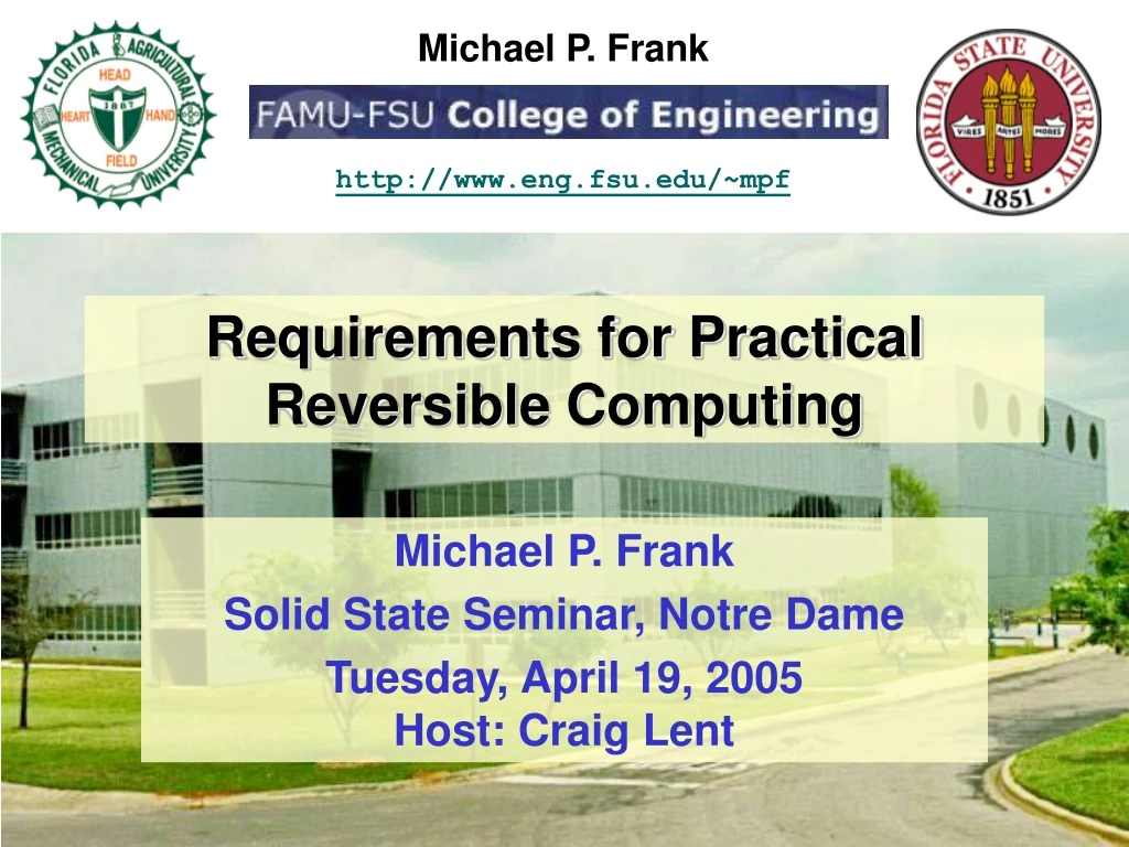
Requirements for Practical Reversible Computing

1. Michael P. Frank http://www.eng.fsu.edu/~mpf Requirements for Practical Reversible Computing Michael P. Frank Solid State Seminar, Notre Dame Tuesday, April 19, 2005Host: Craig Lent

2. Abstract of Talk • I’ll survey requirements for energy-efficient computing beyond the limits of traditional (“irreversible”) computing technologies. • We’ll discuss requirements on devices, logic, and on mechanisms for driving & synchronizing the logic. • Outline of talk: • Brief introduction • Some important device-level figures of merit: • Energy & entropy coefficients, device cost, speed • I’ll also discuss limits on some of these • Logic-level requirements for reversibility: • Not as stringent as traditionally depicted! • I’ll show several ways to generalize the requirements. • Power/clock mechanisms: • Requirements and major challenges • A call to Action! M. Frank, "Requirements for Practical Reversible Computing"

3. Introduction • The Importance of Energy Efficiency • Limits to Energy Efficiency in Conventional Computing • Reversible Computing to the Rescue! M. Frank, "Requirements for Practical Reversible Computing"

4. What is Efficiency? • The efficiencyη of a process that consumes valued resource R and produces valued product P is the ratio between the amount of product produced, and the amount of resource consumed: η = Pprod/Rcons. • Example 1: A heat engine “consumes” (which in this case, means “degrades”) an amount Q of high-temperature heat, and produces an amount W of work. • The heat engine’s efficiency is thus ηh.e. = W/Q. (Dimensionless.) • Carnot showed that ηh.e. ≤ (TH − TL)/TH. • Example 2: A computer consumes an amount Econs of free energy, and performs Nops useful computational operations (produces Nops operations worth of computational “effort”). • The computer’s (energy) efficiency is thus ηE,comp = Nops/Econs. • Units: Operations per unit energy, or ops/sec/watt. M. Frank, "Requirements for Practical Reversible Computing"

5. Energy Efficiency Limits Cost Efficiency! • Of course, there are other economically valuable resources besides energy that are consumed in computing… • Manufacturing/operating costs, opportunity costs, etc. • But, the total cost ¢ of a process obviously can never be less than the cost ¢E of the energy used! • Thus, cost-efficiency FC = Nops/¢ is limited to be at most Nops/¢E, • or, at best proportional to the energy efficiencyηE = Nops/E. •  Greatly improving cost-efficiency requires improving energy efficiency, when energy-related costs are significant! • The direct and indirect costs of energy have always been non-negligible contributors to total operating costs in computing. • The many orders-of-magnitude improvement in computer cost-efficiency over the last 50 years has only been possible because of energy efficiency improvements of comparable magnitude! M. Frank, "Requirements for Practical Reversible Computing"

6. Lower Bounds on Energy Dissipation • In today’s 90 nm VLSI technology, for minimal operations (e.g., conventional switching of a minimum-sized transistor): • Ediss,op is on the order of 1 fJ (femtojoule)  ηE≲ 1015 ops/sec/watt. • Will be a bit better in coming technologies (65 nm, maybe 45 nm) • Conventional digital technologies are subject to several lower bounds on their energy dissipation Ediss,op for digital logic / storage / communication operations, • And thus, corresponding upper bounds on their energy efficiency. • Some of the known bounds include: • Leakage-based limit for high-performance field-effect transistors: • Perhaps roughly ~5 aJ (attojoules)  ηE≲ 2×1017 operations/sec/watt • Reliability-based limit for all non-energy-recovering technologies: • Roughly 1 eV (electron-volt)  ηE≲ 6×1018 operations/sec/watt • von Neumann-Landauer (VNL) bound for all irreversible technologies: • Exactly kT ln 2 ≈ 18 meV ηE≲ 3.5×1020 operations/sec/watt • For systems whose waste heat ultimately winds up in Earth’s atmosphere, • i.e., at temperature T ≈ Troom = 300 K. M. Frank, "Requirements for Practical Reversible Computing"

7. Trend of Min. Transistor Switching Energy Based on ITRS ’97-03 roadmaps fJ Node numbers(nm DRAM hp) Practical limit for CMOS? aJ Naïve linear extrapolation zJ M. Frank, "Requirements for Practical Reversible Computing"

8. Reliability Bound on Logic Signal Energies • Let Esig denote the logic signal energy, • The energy involved in storing, transmitting, or transforming a bit’s worth of digital information. • But note that “involved” does not necessarily mean “dissipated!” • As a result of fundamental thermodynamic considerations, it is required that Esig ≥ kBTsig ln R, • Where kB is Boltzmann’s constant, 1.38×10−12 J/K; • and Tsig is the temperature of the local subsystem carrying the signal; • and R is the reliability factor, i.e., the improbability 1/perr of error. • In non-energy-recovering logic technologies (totally dominant today) • Basically all of the signal energy is dissipated to heat on each operation. • And often additional energy (e.g., short-circuit power) as well. • In this case, minimum sustainable dissipation is Ediss,op≳ kBTenv ln R, • Where Tenv is now the temperature of the waste-heat reservoir • Averages around 300 K (room temperature) in Earth’s atmosphere • For a decent R = 2×1017, this energy is ~40 kT ≈ 1 eV. •  For energy efficiency > 1 op/eV, we mustrecover some of the signal energy. • Rather than dissipating it all to heat with each manipulation of the signal. M. Frank, "Requirements for Practical Reversible Computing"

9. Von Neumann-Landauer Bound • Follows directly from the time-reversibility (invertibility) of all fundamental physical dynamics. • This in turn is implied by the Hamiltonian formulation of mechanics; and the unitarity of quantum mechanics.  Very well-established. • Implies that physical information can never be destroyed! • Only reversibly (mathematically invertibly) transformed! • When we lose or discard a bit’s worth of logical information, • e.g., by erasing or destructively overwriting a bit storage location… • the ‘lost’ information must actually remain in existence, • if in no other form, then as a bit’s worth (k ln 2) of physical entropy. • Entropy simply means unknown information in the physical state. • If the logical bit was originally known (not entropy) • then entropy has increased in this process by ∆S = 1 bit = k ln 2. • The energy in the heat reservoir must be increased by an amount ∆S·Tenv = kTenv ln 2 in order to contain this additional entropy. M. Frank, "Requirements for Practical Reversible Computing"

10. VNL Bound on Energy Dissipation from Information Loss Follows directly from the reversibility of fundamental physics! N physical microstates per logical macrostatebefore bit erasure(shown as 8 for clarity in this simple example) Physicalmicrostatetrajectories Logical state “0”,after operation S = k ln 8 = 3 bits S = k ln 16 = 4 bits Logical state “0”,before operation ∆S = 1 bit= k ln 2 Logical state “1”,before operation Ediss = ∆S·Tenv = kTenv ln 2 S = k ln 8= 3 bits M. Frank, "Requirements for Practical Reversible Computing"

11. Reversible Computing • The basic idea is simply this: • Don’t erase information when performing logic / storage / communication operations! • Instead, just reversibly transform it in place! • When reversible digital operations are implemented using well-designed energy-recovering circuitry, • This can result in local energy dissipation Ediss << Esig, • has been empirically demonstrated by many groups. • and even (in principle) energy dissipation Ediss << kT ln 2! • This has been shown in theory, but we are not yet to the point of demonstrating such low levels of dissipation experimentally. • Achieving this goal requires very careful design, • and verifying it requires very sensitive measurement equipment. M. Frank, "Requirements for Practical Reversible Computing"

12. Device-Level Requirements for Reversible Computing • A good reversible device technology should have: • Low manufacturing cost ¢d per device • Important for good overall cost-efficiency • Low rate of static power dissipation Pleak due to energy leakage. • Required for energy-efficient storage • Low energy coefficientcE = Ediss/f (energy dissipated per operation per unit transition frequency) for adiabatic transitions. • Implies we can achieve a high operating frequency (and thus good cost-performance) at a given level of energy efficiency. • High maximum transition frequency fmax. • Important for those applications in which latency of serial computations dominates total cost • Important: For system-level energy efficiency, Pmin and cE must be taken as effective global values measuring the implied amount of energy emitted into the outside environment at temperature Tenv. • With an ideal (Carnot) refrigerator, Pmin = StTenv and cE = cSTenv, • Where St = the static rate of leakage entropy generation per unit time, • and cS = Sgen/f adiabatic entropy coefficient, or entropy generated per unit transition frequency. M. Frank, "Requirements for Practical Reversible Computing"

13. Energy & Entropy Coefficients in Electronics • For a transition involving the adiabatic transfer of an amount Q of charge along a path with resistance R: • The raw (local) energy coefficient is given bycE = Edisst = Pdisst2 = IVt2 = I2Rt2 = Q2R. • Where V is the voltage drop along the path. • The entropy coefficient cS = Q2R/Tpath. • where Tpathis the local thermodynamic temperature in the path. • Effective (global) energy coefficient cE,eff = Q2R(Tenv/Tpath). • The cE of a simple adiabatic circuit in a recent 180 nm technology (measured in a Cadence simulation) was ~80 eV/GHz. • Corresponds to a Q per charged-up transistor gate of on the order of 6,000 electrons. M. Frank, "Requirements for Practical Reversible Computing"

14. Limiting Cases of Energy/Entropy Coefficients • Entropy/entropy coefficients in adiabatic “single electronics:” • Suppose the amount of charge moved |Q| = q (a single electron) • Let the path consist of a single quantum channel (chain of states) • Has quantum resistanceR = R0 = 1/G0 = h/2q2 = 12.9 kΩ. • Then cE = h/2 = 2.07 meV/THz (very low!) • If path is at Tpath = Troom = 300 K, then cS = 0.08 k/THz. • For N× better efficiency than this, let the path consist of N parallel quantum channels.  N×lower resistance. • What about systems where resistive models may not apply? • E.g., superconductors, photonics, etc. • A more general and rigorous (but perhaps loose) lower bound on the energy coefficient in all adiabatic quantum systems is given by the expression cE ≥ h2/4Egt, • where Eg = energy gap between ground & excited states, • and t = time taken for a single orthogonalizing transition • Ex.: Let Eg = 1 eV, t = 1 ps. Then cE ≥ 4.28 μeV/THz. M. Frank, "Requirements for Practical Reversible Computing"

15. Logic-Level Requirements for Reversible Computing • A traditional logical “requirement” for thermodynamically reversible logic: • All local n-bit operations must carry out a 1-to-1 (bijective) transformation on the space of all 2n possible inputs. • Strictly speaking, this is false! • It is actually quite a bit more restrictive than necessary. • Avoiding Landauer’s principle only requires: • The number of states in the possible set (consistent with our design knowledge) must not decrease. • But many-to-many, not just 1-to-1 transistions may be used. • Further, this is only required to be true on average. • E.g., it is OK to erase previously nondeterministically obtained bits! • Finally, it is only required to be true on states encountered, • Not necessarily on the space of all2n describable inputs! M. Frank, "Requirements for Practical Reversible Computing"

16. Non-Injective Operations Can Be Thermodynamically Reversible • For example, consider the “operation”illustrated at right. • 3 initial states • all equally likely • 3 final states • Transition relation is not an injective function, • but a many-to-many relation (may have weighted arcs) • As long as the transition probabilities have semi-detailed balance (a: ∑bp(ba) = 1),initially uniform distributions will stay that way! • No increase in entropy, if initial state is unknown. (Circlescontainstateproba-bilities.) M. Frank, "Requirements for Practical Reversible Computing"

17. Reversible Computations Can Even Contain Many-to-One Operations • As long as operations are still N-to-N on average! • E.g., in the pictured computation, we first nondeterministically randomize a known bit • Extracting 1 bit of entropy from the environment • then later, we erase this bit, • Returning the bit of entropy to the environment. • Total entropy need not increase in such a process! (Circlescontainstateproba-bilities.) 1/2 1 1 1/2 M. Frank, "Requirements for Practical Reversible Computing"

18. We are even free to permanently compress parts of the state space… • As long as the subset of states that actually arise is not compressed! • E.g., at right, the operation takesthe top two initial states to thesame final state… • But we design the system in such a way that those two states never arise! • Note the state that can arise has a unique successor… • More generally, its “equivalent set” (set of equivalent states) must not be compressed. 0 0 0 1 1 (Circlescontainstateproba-bilities.) M. Frank, "Requirements for Practical Reversible Computing"

19. Pop Quiz: Can This Machine Be Thermodynamically Reversible? • Suppose the transition relation between digital states is as shown. • Outgoing arcs are chosen with equal weight. • Subset A of initial states is guaranteed, by design, never to arise. • States in subsets B and C may arise, but the particular state within a given subset is completely random. A B C Answer: Yes, in fact, running thismachine can (temporarily) decrease the entropy of the environment! M. Frank, "Requirements for Practical Reversible Computing"

20. Why is all of this Useful? • The fact that only N-to-N (not 1-to-1) ops are required is useful because: • We can encode known information using “equivalent sets” of lower-level states whose transitions are treated as noninjective (and nondeterministic). • That is, we don’t have to track the complete microstate. • The fact that transitions only need to be N-to-Non average is useful because: • It allows us to execute randomized algorithms, • and dispose of the random numbers later, when we no longer need them. • The fact that only the possible subset needs to be reversible is useful because: • It allows us to build fully-reversible machines out of easily-implemented logic devices that are only conditionally reversible. • That is, that are reversible only if certain design rules are followed. • The resulting designs can be much simpler! • Compared to building everything from Toffoli and Fredkin gates. M. Frank, "Requirements for Practical Reversible Computing"

21. Other Misconceptions To Avoid in Reversible Logic Designs • Be aware that quantum and reversible “logic networks” (time-sequences of operations) are not the same thing as hardware diagrams! • It’s generally a bad idea to try to use one directly as the other. • Please always take care to distinguish between logic operations and logic gates. • Operations are transformations of part of the logical state, • and their “inputs” and “outputs” are really just the “before” and “after” configurations of the local state. • Gates are physical devices (hardware) that can implement one or more operations on their set of impinging wires (I/O signals). • For hardware, an “input” means a wire that affects the gate’s behavior, • and an “output” means a wire that the gate’s behavior affects. • A gate may use some signal wires as both inputs and outputs! • E.g., a reversible operation depicted as having 3 inputs and 3 outputs can be implemented by a physical gate that is attached to a total of only 3 wires. M. Frank, "Requirements for Practical Reversible Computing"

22. What’s the Simplest Universal Reversible Logic Gate? • Where “simplest” here refers to number of data signals operated on… • Guess what: It isn’t the Fredkin or Toffoli gate… • And it isn’t any of the fully-reversible gates! • Rather it’s a conditionally reversible gate… • I call it the reversible buffer, or crSET/crCLR gate: • It involves only 2 data signals: • 1 input, and 1 output (can be tristated) • Some implementations use only 2 CMOS transistors! • Together with latches, we can efficiently build arbitrary reversible logic with it. M. Frank, "Requirements for Practical Reversible Computing"

23. Reversible Buffers and Latches • A universal set of conditionally reversible operations: • crSET(a,b): Controlled Reversible SET. • Semantics: (ab = 0) if a then b := 1, else if b then unlock(a), else lock(a) • If a is 1, then set b to 1 (else leave b alone). • Reversible on condition that a and b are not both 1 (& locks are obeyed). • crCLR(a,b): Controlled Reversible CLR. • A.k.a. crUnSET – It’s crSET in reverse. • Semantics: (ab = 0) if a then b := 0, else if b then lock(a), else unlock(a) • If a is 1, then set b to 0. • Reversible if we don’t have a = 1, b = 0 (& locks are obeyed) • rLatch(a,b): Reversible latch operation. • Semantics: a =/= b • Meaning, break the connection a from b through this particular latch HW. • rUnLatch(a,b): Reversible “unlatch” operation. • Semantics: (a = b) a == b • Meaning, connect a to b through a particular bit of latching HW. • Reversible on condition that a = b initially. M. Frank, "Requirements for Practical Reversible Computing"

24. CMOS Gate Implementating crSET & crCLR • Reversible Buffer (does crSET & crCLR) Implementation Icon Spacetime Diagram drive crSET crCLR in out in (CMOS transmissiongate) inNP or 2 drive 0 0 out out in out (in) time drive inP • Double the hardware to get a dual-rail output • Can show timing control signal “drive” on icon • Special notation in spacetime diagram is used to keep track of constraints on nodes. inNP inN 2 out M. Frank, "Requirements for Practical Reversible Computing"

25. CMOS Gate Implementing rLatch/rUnLatch • Symmetric Reversible Latch Implementation Icon Spacetime Diagram crLatch crUnLatch connect in mem in 2 mem in or connect (in) mem in mem time • Just a transmission gate again • This time controlled by a clock, with the data signal driving • Concise, symmetric hardware icon – Just a short orthogonal line • Thin strapping lines denote connection in spacetime diagram. M. Frank, "Requirements for Practical Reversible Computing"

26. Example: Building cNOT from rlXOR • rlXOR(a,b,c): Reversible latched XOR. • Semantics: (c = N) c := ab. • Given that c is initially in a predefined “neutral” or “no information” state N, set c to the value (a XOR b). • Easy to implement with transistors (or in QCA) • cNOT(a,b): Controlled-NOT operation. • Semantics: b := ab. (No preconditions.) • A popular “primitive” in reversible & quantum comp. • Complex to implement in hardware • Not a very good building block for practical hardware! • But we can build it, if we really want to. M. Frank, "Requirements for Practical Reversible Computing"

27. cNOT from rlXOR: Hardware Diagram • A logic block implementing an in-place cNOT operation (a cNOT “gate”) can be constructed from 2 rlXOR gates and two latched buffers. • The key is: • Operate some of the gates in reverse! Reversiblelatches A B X M. Frank, "Requirements for Practical Reversible Computing"

28. Simulation Results from Cadence <.01× the power @ 1 MHz >100× faster @ 1 pW/T • Assumptions & caveats: • Assumes ideal trapezoidal power/clock waveform. • Minimum-sized devices, 2λ×3λ* .18 µm (L) × .24 µm (W) • nFET data is shown* pFETs data is very similar • Various body biases tried * Higher Vth suppresses leakage • Room temperature operation. • Interconnect parasitics have not yet been included. • Activity factor (transitions per device-cycle) is 1 for CMOS, 0.5 for 2LAL in this graph. • Hardware overhead from fully- adiabatic design style is not yet reflected * ≥2× transistor-tick hardware overhead in known reversible CMOS design styles 1 nJ 100 pJ Standard CMOS 10 pJ 10 aJ 1 pJ 1 aJ 1 eV Energy dissipated per nFET per cycle 100 fJ 2V 100 zJ 2LAL 1.8-2.0V 1V 10 fJ 10 zJ 0.5V 0.25V 1 fJ kT ln 2 1 zJ 100 aJ 100 yJ M. Frank, "Requirements for Practical Reversible Computing"

29. O(log n)-time carry-skip adder S A B S A B S A B S A B S A B S A B S A B S A B G Cin GCoutCin GCoutCin G Cin GCoutCin G Cin GCoutCin G Cin P P P P P P P P PmsGlsPls Pms GlsPls PmsGlsPls Pms GlsPls MS MS LS LS G G GCout Cin GCout Cin P P P P Pms GlsPls Pms GlsPls MS LS G GCout Cin P P Pms GlsPls LS GCout Cin P With this structure, we can do a2n-bit add in 2(n+1) logic levels→ 4(n+1) reversible ticks→ n+1 clock cycles.Hardwareoverhead is<2× regularripple-carry. (8 bit segment shown) 3rd carry tick 2nd carry tick 4th carry tick 1st carry tick M. Frank, "Requirements for Practical Reversible Computing"

30. 32-bit Adder Simulation Results 20x better perf.@ 3 nW/adder 1V CMOS 1V CMOS 0.5V CMOS 0.5V CMOS 2V 2LAL, Vsb=1V 2V 2LAL, Vsb=1V (All results normalized to a throughput level of 1 add/cycle) M. Frank, "Requirements for Practical Reversible Computing"

31. Plenty of Room forDevice Improvement Power per device, vs. frequency • Recall, irreversible device technology has at most ~3-4 orders of magnitude of power-performance improvements remaining. • And then, the firm kT ln 2 limit is encountered. • But, a wide variety of proposed reversible device technologies have been analyzed by physicists. • With theoretical power-performance up to 10-12 orders of magnitude better than today’s CMOS! • Ultimate limits are unclear. .18µm CMOS .18µm 2LAL k(300 K) ln 2 Variousreversibledevice proposals M. Frank, "Requirements for Practical Reversible Computing"

32. Requirements for Energy-Recovering Clock/Power Supplies • All known reversible computing schemes require a periodic global signal that synchronizes and drives adiabatic transitions. • For good system-level energy efficiency, this signal must oscillate resonantly and near-ballistically, with a high effective quality factor. • Several factors make the design of a satisfactory resonator quite difficult: • Need to avoid uncompensated back-action of logic on resonator • In some resonators, Q factor may scale unfavorably with size • Effective quality factor problem • I’m not saying it’s impossible… • But it’s definitely a nontrivial hurdle, that we need to face up to, pretty urgently… • If we want to convince people that reversible computing will work. M. Frank, "Requirements for Practical Reversible Computing"

33. The Back-Action Problem • The ideal resonator signal is a pure periodic signal. • A pretty general result from communications theory: • A resonator’s quality factor is inversely proportional to its signal bandwidth B. • E.g., for an EM cavity w. resonant frequency ω0, • the half-maximum BW is B = ∆ω = ω0/(2πQ) [1]. • Thus Q∞  B 0. • There must be little or no information in the resonator signal! • However, if the logic load being driven varies from on cycle to the next, • whether due to data-dependent variations, • or structural variations (different amounts of logic being driven per cycle) • this will tend to produce impedance nonuniformities, which will lead to nonuniform reflections of the resonator signal • and thereby introduce nonzero bandwidth into that signal. • Even more generally, any departure of resonator energy away from an ideal desired trajectory represents a form of effective energy dissipation! • we must control exactly where (into what states) all the energy goes • the set of possible microstates of the system must not grow quickly [1] Schwartz, Principles of Electrodynamics, Dover, 1972. M. Frank, "Requirements for Practical Reversible Computing"

34. Unfavorable Scaling of Resonator Quality Factor with Size? • I don’t yet have a perfectly clear and general understanding of this issue, but… • In a lot of oscillator systems I’ve looked at, the resonator Q factor may tend to get worse (or at least, not much better) as the resonator gets smaller. • In LC oscillators, inductor Q scales inversely to frequency • EM emission is greater at high frequencies • But, the tendency is for low f large coil sizes • Anecdotal reports from people working in NEMS community… • Difficult to get high Q in nanoscale electromechanical resonators • Perhaps due to difficulty of precision engineering at nanoscale? • Our own experience working with transmission-line resonators • Example: In a cubical EM cavity of size L, • We have 2πQ = L / 8δ, where δ = skin depth. ([1] again) • Skin depth δ = (2πσk)−1/2, where σ = wall conductivity, k = wave #. • So if L is fixed, high Q small δ  large k  high f  low Q in logic! M. Frank, "Requirements for Practical Reversible Computing"

35. The Effective Quality Factor Problem • Actual quality factor of resonator Q = Eres/Edissr. • Where Eres = energy contained in resonator signal • and Edissr = energy dissipated in resonator per cycle. • But the effective quality factor, for purposes of doing energy-efficient logic transitions is Qeff = Edeliv/Edissr. • Where Edeliv = energy delivered to the logic per transition. • Since 1/Qeff of the logic signal energy is dissipated per cycle. • Thus, Qeff = Q · (Edeliv/Eres). • That is, the effective Q is taken down by the fraction of resonator energy delivered to the logic per cycle. • If a resonator needs to be large to attain high Q, • it may also hold a large amount of energy Eres, • and so it may not have a very high effective Q for driving the logic! M. Frank, "Requirements for Practical Reversible Computing"

36. MEMS (& NEMS) Resonators • State of the art of technology demonstrated in lab: • Frequencies up to the 100s of MHz, even GHz • Q’s >10,000 in vacuum, several thousand even in air! • An important emerging technology being exploredfor use in RF filters, etc., in communicationsSoCs, e.g. for cellphones. U. Mich., poly, f=156 MHz, Q=9,400 34 µm M. Frank, "Requirements for Practical Reversible Computing"

37. Original Concept PATENT PENDING • Imagine a set of charged plates whose horizontal position oscillates between two sets of interdigitated fixed plates. • Structure forms a variable capacitor and voltage divider with the load. • Capacitance changes substantially only when crossing border. • Produces nearly flat-topped (quasi-trapezoidal) output waveforms. • The two output signals have opposite phases (2 of the 4 φ’s in 2LAL) Logicload #2 Logicload #1 V1 V2 RL RL CL CL x t V1 V2 t t M. Frank, "Requirements for Practical Reversible Computing"

38. PATENT PENDING Resonator Schematic Actuator Sensor Sensor Sensor Sensor Actuator M. Frank, "Requirements for Practical Reversible Computing"

39. New Comb Finger Shape IV PATENT PENDING Moving metal plate support arm/electrode Moving plate Range of Motion Arm anchored to nodal points of fixed-fixed beam flexures,located a little ways away, in both directions (for symmetry) … z y Phase 180° electrode Phase 0° electrode Repeatinterdigitatedstructurearbitrarily manytimes along y axis,all anchored to the same flexure x C(θ) C(θ) 0° 360° 0° 360° θ θ M. Frank, "Requirements for Practical Reversible Computing"

40. Another Candidate Layout PATENT PENDING M. Frank, "Requirements for Practical Reversible Computing"

41. New simulation results M. Frank, "Requirements for Practical Reversible Computing"

42. Serpentine spring Front-side view Proof mass Comb drive Back-side view DRIE CMOS-MEMS Resonators 150 kHz Resonators M. Frank, "Requirements for Practical Reversible Computing"

43. Post-TSMC35 AdiaMEMS Resonator PATENT PENDING Taped out April ‘04 Drivecomb Sensecomb Flexarm M. Frank, "Requirements for Practical Reversible Computing"

44. A Challenge for Our Community • I predict that the field’s critics will never be silenced by theory and simulations alone… • To prove to the world that reversible computing can really work will require a complete empirical demonstration. • We also cannot afford to sweep resonator-related difficulties under the rug… • A convincing demonstration of low total system power must be completely self-contained, including the resonator. • with only DC power input as needed to keep it running • My challenge to us: • Let’s work together to fabricate and empirically demonstrate (for starters) an N-bit binary counter that measurably dissipates less than some small multiple of kT energy per cycle in a room-T environment • “Wall-plug” power, as our critics like to put it. M. Frank, "Requirements for Practical Reversible Computing"

45. Why a Binary Counter? • The number of bits that must flip varies dramatically from cycle to cycle. • Usually just 1 or 2, sometimes as many as N. • The average number is small, however… • conventional irreversible solutions would need to dissipate only a small multiple of the bit energy per cycle on average. • Data-dependent: Depends on initial state of the counter. • The resonator system cannot “know” what the counter state is • As a result, the physical action required to carry out each cycle is non-uniform, and data-dependent. • Implies that either the energy supplied is non-uniform, or the time taken per cycle is non-uniform. • Either one poses challenges for resonator design. • I believe this goal is already quite difficult, • but is a good stepping-stone towards a full reversible CPU. M. Frank, "Requirements for Practical Reversible Computing"

46. Conclusion • Reversible computing is a prerequisite for getting beyond the next decade or so of improvements in computer energy efficiency. • This is rigorously implied by fundamental physics! • Practical reversible computing requires: • Devices with very low energy coefficients cE… • e.g., Notre Dame’s own Quantum-dot Cellular Automata • Logic design that is somewhat constrained • though not as much as people used to think! • Very high quality power/clock resonator systems • this is, I think, by far the most difficult part to achieve • Let’s work together to tackle the engineering challenges and convincingly demonstrate this new paradigm for 21st-century computing! M. Frank, "Requirements for Practical Reversible Computing"

47. The 1st International Workshop on Reversible Computing (RC’05) • A special session in the ACM Computing Frontiers conference (CF’05). • To be held in Ischia, Italy, May 4-6, 2005. • Speakers include: • Averin, Bennett, DeBenedictis, Forsberg, Frank, Fredkin, Frost, Semenov, Toffoli, Vitanyi… (& others) • Workshop website: • http://www.eng.fsu.edu/~mpf/CF05/RC05.htm M. Frank, "Requirements for Practical Reversible Computing"