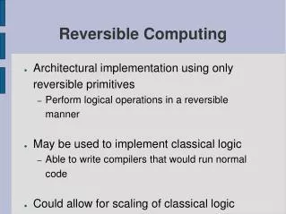
Reversible Computing
Reversible Computing. Michael P. Frank University of Florida Departments of CISE and ECE mpf@cise.ufl.edu Simons Conference Lecture Stony Brook, New York May 28-31, 2003. Quantum Computing’s Practical Cousin. Abstract.

Reversible Computing
E N D
Presentation Transcript
Reversible Computing Michael P. FrankUniversity of FloridaDepartments of CISE and ECE mpf@cise.ufl.edu Simons Conference LectureStony Brook, New YorkMay 28-31, 2003 Quantum Computing’s Practical Cousin
Abstract • “Mainstream” quantum computing is very difficult, and its currently known applications are quite limited. • Focus is on maintaining coherence of global superpositions. • Reversible computing is much easier, and its long-term practical applications are almost completely general. • Its benefits are provable from fundamental physics. • Well-engineered reversible computers might yield general, ≥1,000× cost-efficiency benefits by 2055. • We outline how this projection was obtained. • More attention should be paid to implementing self-contained, reversible, ballistic device mechanisms. • We give requirements, proof-of-concept examples.
Organization of Talk • Reversible Computing (RC) vs. Quantum Computing (QC) • Fundamental Physical Limits of Computing • Models and Mechanisms for RC • Nanocomputer Systems Engineering & the Cost-Efficiency Benefits of RC • Conclusion: RC is a good area to be in!
Part I Reversible Computing versus Quantum Computing
QM, Decoherence & Irreversibility • Everett & (more recently) Zurek taught us why it is not inconsistent w. our observations to view quantum evolution as always being completely unitary “in reality.” • What about apparent wavefunction collapse, decoherence, and thermodynamic irreversibility (entropy generation)? • All can be viewed as “just” symptoms of our practical inability to keep track of the full quantum evolution, w. all correlations & entanglements that get created between interacting subsystems. (Also cf. Jaynes ’57) Presumed ‘true’ underlying reality: Approximate model often used: SubsystemA SubsystemB SubsystemA SubsystemB U ~U Densitymatrices ρA ρB Global pure state ΨAB
Quantum Computing • Relies on coherent, global superposition states • Required for speedups of quantum algorithms, but… • Cause difficulties in scaling physical implementations • Invokes externally-modulated Hamiltonian • Low total system energy dissipation is not necessarily guaranteed, if dissipation in control system is included • Known speedups for only a few problems so far… • Cryptanalysis, quantum simulations, unstructured search, a small handful of others. Progress is hard… • QC might not ever have very much impact on the majority of general-purpose computing.
Reversible Computing • Requires only an approximate, local coherence of ‘pointer’ states, & direct transitions between them • Ordinary signal-restoration plus classical error correction techniques suffice; fewer scaling problems • Emphasis is on low entropy generation due to quantum evolution that is locally mostly coherent • Requires we also pay attention to dissipation in the timing system, integrate it into the system model. • Benefits nearly all general-purpose computing • Except fully-serial, or very loosely-coupled parallel, when the cost of free energy itself is also negligible.
Part II The Fundamental Physical Limits of Computing
Fundamental Physical Limits of Computing ImpliedUniversal Facts Affected Quantities in Information Processing Thoroughly ConfirmedPhysical Theories Speed-of-LightLimit Communications Latency Theory ofRelativity Information Capacity UncertaintyPrinciple Information Bandwidth Definitionof Energy Memory Access Times QuantumTheory Reversibility 2nd Law ofThermodynamics Processing Rate Adiabatic Theorem Energy Loss per Operation Gravity
s″0 s0 0 0 Landauer’s 1961 Principle from basic quantum theory Before bit erasure: After bit erasure: Ndistinctstates … … … sN−1 s″N−1 0 0 2Ndistinctstates Unitary(1-1)evolution s′0 s″N 1 0 Ndistinctstates … … … … s′N−1 s″2N−1 1 0 Increase in entropy: S = log 2 = k ln 2. Energy lost to heat: ST = kT ln 2
Part III Reversible ComputingModels & Mechanisms
Bistable Potential-Energy Wells • Consider any system having an adjustable, bistable potential energy surface (PES) in its configuration space. • The two stable states form a natural bit. • One state represents 0, the other 1. • Consider now the P.E. well havingtwo adjustable parameters: • (1) Height of the potential energy barrierrelative to the well bottom • (2) Relative height of the left and rightstates in the well (bias) 0 1 (Landauer ’61)
Possible Parameter Settings • We will distinguish six qualitatively different settings of the well parameters, as follows… BarrierHeight Direction of Bias Force
One Mechanical Implementation Stateknob Rightwardbias Barrierwedge Leftwardbias spring spring Barrier up Barrier down
Possible Adiabatic Transitions (Ignoring superposition states.) • Catalog of all the possible transitions in these wells, adiabatic & not... “1”states 1 1 1 leak 0 “0”states 0 leak 0 BarrierHeight N 1 0 Direction of Bias Force
Ordinary Irreversible Logics • Principle of operation: Lower a barrier, or not, based on input. Series/parallel combinations of barriers do logic. Major dissipation in at least one of the possible transitions. 1 Input changes, barrier lowered 0 • Amplifies input signals. Example: Ordinary CMOS logics Outputirreversiblychanged to 0 0
Ordinary Irreversible Memory • Lower a barrier, dissipating stored information. Apply an input bias. Raise the barrier to latch the new informationinto place. Remove inputbias. Retractinput 1 1 Dissipationhere can bemade as low as kT ln 2 Retractinput Barrierup 0 0 Barrier up Input“1” Input“0” Example:DRAM N 1 0
Input-Bias Clocked-Barrier Logic Can amplify/restore input signalin the barrier-raising step. • Cycle of operation: • (1) Data input applies bias • Add forces to do logic • (2) Clock signal raises barrier • (3) Data input bias removed (3) 1 1 (4) Can reset latch reversibly (4) given copy ofcontents. (3) 0 0 (2) (4) (4) (4) (2) Examples: AdiabaticQDCA, SCRL latch, Rod logic latch, PQ logic,Buckled logic (1) (1) N 1 0 (4) (4)
Input-Barrier, Clocked-Bias Retractile • Barrier signal amplified. • Must reset output prior to input. • Combinational logic only! • Cycle of operation: • Inputs raise or lower barriers • Do logic w. series/parallel barriers • Clock applies bias force which changes state, or not 0 0 0 (1) Input barrier height Examples:Hall’s logic,SCRL gates,Rod logic interlocks N 1 0 (2) Clocked force applied
Input-Barrier, Clocked-Bias Latching • Cycle of operation: • Input conditionally lowers barrier • Do logic w. series/parallel barriers • Clock applies bias force; conditional bit flip • Input removed, raising the barrier &locking in the state-change • Clockbias canretract 1 (4) (4) 0 0 0 (2) (2) (3) (1) Examples: Mike’s4-cycle adiabaticCMOS logic (2) (2) N 1 0
Full Classical-Mechanical Model Sleeve The following components are sufficient for a complete, scalable, parallel, pipelinable, linear-time, stable, classical reversible computing system: (a) Ballistically rotating flywheel driving linear motion. (b) Scalable mesh to synchronize local flywheel phases in 3-D. (c) Sinusoidal to flat-topped waveform shape converter. (d) Non-amplifying signal inverter (NOT gate). (e) Non-amplifying OR/AND gate. (f) Signal amplifier/latch. (a) (c) (b) (f) (d) Primary drawback: Slow propagationspeed of mechanical (phonon) signals. (e) cf. Drexler ‘92
A MEMS Supply Concept • Energy storedmechanically. • Variable couplingstrength → customwave shape. • Can reduce lossesthrough balancing,filtering. • Issue: How toadjust frequency?
MEMS/NEMS Resonators • State of the art of technology demonstrated in lab: • Frequencies up to the 100s of MHz, even GHz • Q’s >10,000 in vacuum, several thousand even in air • Rapidly becoming technology of choicefor commercial RF filters, etc., in communicationsSoC (Systems-on-a-Chip) e.g. for cellphones.
Graphical Notation for Reversible Circuits • Based on analogy with earlier mechanical model • Source for a flat-topped resonant signal • Cycle length of n ticks • Rises from 0→1 during tick #r • Falls from 1→0 during tick #f • Signal path with 1 visualized as displacement along path in direction of arrow: • Non-amplifying inverter: • Non-amplifying OR:
Graphical Notation, cont. • Interlock (Amplifier/Latch): • If gate knob is lowered (1) then a subsequent 0→1 signal from the left will be passed through to the right, otherwise not. • Simplified “electroid” symbol (Hall, ‘92) gate
P 2LAL: 2-level Adiabatic Logic (Implementable using ordinary CMOS transistors) P P • Use simplified T-gate symbol: • Basic buffer element: • cross-coupled T-gates • Only 4 timing signals,4 ticks per cycle: • i rises during tick i • i falls during tick i+2 mod 4 : 1 Tick # in 0 1 2 3 0 1 out 2 0 3
2LAL Cycle of Operation Tick #0 Tick #1 Tick #2 Tick #3 11 in1 in0 10 out1 in 01 00 11 in=0 out0 out=0 01 00
2LAL Shift Register Structure 1 2 3 0 • 1-tick delay per logic stage: • Logic pulse timing & propagation: in out 0 1 2 3 0 1 2 3 ... 0 1 2 3 ... in in
More complex logic functions • Non-inverting Boolean functions: • For inverting functions, must use quad-rail logic encoding: • To invert, justswap the rails! • Zero-transistor“inverters.” A B A A B AB AB A = 0 A = 1 A0 A0 A1 A1
Reversible / Adiabatic Chips Designed @ MIT, 1996-1999 By the author and other then-students in the MIT Reversible Computing group,under AI/LCS lab members Tom Knight and Norm Margolus.
Part IV Nanocomputer Systems Engineering: Analyzing & Optimizing the Benefits of Reversible Computing
Cost-Efficiency:The Key Figure of Merit • Claim: All practical engineering design-optimization can ultimately be reduced to maximization of generalized, system-level cost-efficiency. • Given appropriate models of cost “$”. • Definition of the Cost-Efficiency %$ of a process: %$ :≡$min/$actual • Maximize %$ by minimizing $actual • Note this is valid even when $min is unknown
Important Cost Categories in Computing Focus of mosttraditionaltheory aboutcomputational“complexity.” • Hardware-Proportional Costs: • Initial Manufacturing Cost • Time-Proportional Costs: • Inconvenience to User Waiting for Result • (HardwareTime)-Proportional Costs: • Amortized Manufacturing Cost • Maintenance & Operation Costs • Opportunity Costs • Energy-Proportional Costs: • Adiabatic Losses • Non-adiabatic Losses From Bit Erasure • Note: These may both vary independently of (HWTime)! These costsmust be included also in practicaltheoreticalmodels ofnanocomputing!
Logic Devices Technology Scaling Interconnections Synchronization Processor Architecture Capacity Scaling Energy Transfer Programming Error Handling Performance Cost Computer Modeling Areas An Optimal, Physically Realistic Model of Compu-ting Must Accurately Address All these Areas!
Important Factors Included in Our Model • Entropic cost of irreversibility • Algorithmic overheads of reversible logic • Adiabatic speed vs. energy-loss tradeoff • Optimized degree of reversibility • Limited quality factors of real devices • Communications latencies in parallel algorithms • Realistic heat flux constraints
Technology-Independent Model of Nanoscale Logic Devices Id – Bits of internal logical state information per nano-device Siop – Entropy generated per irreversible nano-device operation tic – Time per device cycle (irreversible case) Sd,t – Entropy generated per device per unit time (standby rate, from leakage/decay) Srop,f – Entropy generated per reversible op per unit frequency d – Length (pitch) between neighboring nanodevices SA,t – Entropy flux per unit area per unit time
Reversible Emulation - Ben89 k = 2n = 3 k = 3n = 2
Technological Trend Assumptions Entropy generatedper irreversible bittransition, nats Absolute thermodynamiclower limit! Minimum pitch (separation between centers of adjacent bit-devices), meters. Nanometer pitch limit Minimum time perirreversible bit-devicetransition, secs. Example quantum limit Minimum cost perbit-device, US$.
Fixed Technology Assumptions • Total cost of manufacture: US$1,000.00 • User will pay this for a high-performance desktop CPU. • Expected lifetime of hardware: 3 years • After which obsolescence sets in. • Total power limit: 100 Watts • Any more would burn up your lap. Ouch! • Power flux limit: 100 Watts per square centimeter • Approximate limit of air-cooling capabilities • Standby entropy generation rate: 1,000 nat/s/device • Arbitrarily chosen, but achievable
Cost-Efficiency Benefits Scenario: $1,000/3-years, 100-Watt conventional computer, vs. reversible computers w. same capacity. ~100,000× ~1,000× Best-case reversible computing Bit-operations per US dollar Worst-case reversible computing Conventional irreversible computing All curves would →0 if leakage not reduced.
Lower Limit to Entropy Generation Per Bit-Operation • Scaling withdevice’s quantum“quality” factor q. • The optimal redundancyfactor scales as: 1.1248(ln q) • The minimumentropy gener-ation scales as:q −0.9039
Conclusions • Reversible Computing is related to, but much easier to accomplish than Quantum Computing. • The case for RC’s long-term, general usefulness for future practical, real-world nanocomputer engineering is now fairly solid. • The world has been slow to catch on to the ideas of RC, but it has been short-sighted… • RC will be the foundation for most 21st-century computer engineering.
Reversible By Michael Frank Reversible Computing To besubmittedtoScientificAmerican: With device sizes fast approaching atomic-scale limits, ballistic circuits that conserve information will offer the only possible way to keep improving energy efficiency and therefore speed for most computing applications.