Reversible Computing A Brief Introduction
Reversible Computing A Brief Introduction. Dr. Michael P. Frank mpf@cise.ufl.edu Dept. of Computer & Information Science & Engineering (Affil. Dept. of Electrical & Computer Engineering) University of Florida, Gainesville, Florida. Presented at:

Reversible Computing A Brief Introduction
E N D
Presentation Transcript
Reversible ComputingA Brief Introduction Dr. Michael P. Frankmpf@cise.ufl.eduDept. of Computer & Information Science & Engineering(Affil. Dept. of Electrical & Computer Engineering)University of Florida, Gainesville, Florida Presented at: 2004 Computing Beyond Silicon Summer School (Week 4)California Institute of Technology Pasadena, California, July 6-8, 2004
Abstract • The performance of power-limited computing systems is directly limited by the energy efficiency of logic operations. Performance (ops / time) = Power (energy dissipated / time) × Energy efficiency (ops / energy dissipated) • Traditional logic techniques are approaching a number of very general physical limits on energy efficiency. • Due to quite fundamental thermodynamic considerations. • The only potential way to circumvent all of these limits is through (logically & physically) reversible computing (RC). • It is related to quantum computing, but easier in some ways. • RC appears to be doable, but it is still very challenging… • But, it is a challenge that we must meet, for continued progress. • In this talk, we survey fundamental concepts, available technologies, and outstanding problems of RC.
Moore’s Law – Devices per IC Intel µpu’s Early Fairchild ICs
Device Size Scaling Trends Based on ITRS ’97-03 roadmaps (1 µm) Virus Protein molecule Naïve linear extrapolations Effective gate oxide thickness DNA/CNT radius Silicon atom Hydrogen atom
Trend of Minimum Transistor Switching Energy Based on ITRS ’97-03 roadmaps fJ Practical limit for CMOS? aJ Naïve linear extrapolation zJ
The Leakage Problem • The primary traditional approach to decrease energy dissipation per logic-op has been: • Simply decrease the magnitude of the ½CV2 energy that is stored per bit. • This is done by moving to smaller transistor structures, which decreases C and usable V. • However, as V decreases, there is a problem. • An upper bound on the on/off ratio Ron/off = Ion/Ioff of transistors is given by the relation log Ron/off≲V/s. • The parameter s is called the subthreshold slope. • Typical units: mV/decade (decade = log 10) • The exact value of s depends on the precise device geometry, • It is reduced by going to multi-gate or surround-gate structures. • But, s has a fundamental room-temperature T minimum of s ≥ T/q = (kT/q ln 10)/decade ≈ 60 mV/decade in FETs, independent of materials! (Whether carbon nanotubes, Si nanowires, etc. • This is just due to the ratio between above-barrier state occupancy probabilities for a change in barrier height of V. (From Boltzmann distrib.) • At low voltages (e.g., a few hundred mV), transistors can’t turn off effectively, and there is substantial continuous power dissipation. • Leakage already accounts for as much as 40% of total power in many designs!
A Fairly Conventional “Optimistic” Technology Scenario for CMOS • Suppose device lengths are cut in half every 3 years… • From 90 nm today down to 22 nm node in 2010 (then stop). • Node capacitances, gate delays also decrease accordingly… • “Technology boosters” such as high-κ dielectrics & novel FET structures (FinFET, surround-gate, etc.) keep leakage power manageable, for a little while… • However, the absolute minimum room-T subthreshold slope for FETs will remain 60 mV/decade! (= (kT/q)/log 10) • Assume this point is also reached by around 2007. • Voltages then reach a minimum of ~0.5V in 2007. • Can’t go lower while keeping on/off ratio above 108 level! • A minimum level chosen so as to keep leakage small • Now, consider what all this implies about future chip performance, given a 100 W maximum power level… • Let max raw performance = 100 W / (½CV2 gate energy)
Not much life left for standard CMOS… e.g. 825 million devices actively switching @ 4 GHz, ~7,000 kT dissip. per device-op e.g., 67 million devices actively switching @ 3 GHz Now, even if the leakage problem were solved, the ~100 kTlimit for reliable switching is only another factor of 70 beyond this point!
Reversible Computing Motivation & Basic Concepts
s0 t0 0 0 (Was hinted at by von Neumann ’49) Landauer’s (1961) principle:The minimum energy cost of oblivious bit erasure Before bit erasure: After bit erasure: Npossibledistinctstates … … … sN−1 tN−1 2Npossibledistinctstates 0 0 Unitary(one-to-one)evolution s′0 tN 1 0 Npossibledistinctstates … … … … s′N−1 t2N−1 1 0 Increase in entropy: ∆S = log 2 = k ln 2. Energy dissipated to heat: T∆S = kT ln 2
Non-oblivious “erasure” (by decomputing known bits) avoids the von Neumann–Landauer bound Before decomputing B: After decomputing B: A B A B s0 t0 0 0 0 0 Npossibledistinctstates Npossibledistinctstates … … … A B A B sN−1 tN−1 0 0 0 0 Unitary(one-to-one)evolution A B A B s′0 t′0 1 1 1 0 Npossibledistinctstates Npossibledistinctstates … … … … A B A B s′N−1 t′N−1 1 1 1 0 Increase in entropy: ∆S→ 0. Energy dissipated to heat: T∆S → 0
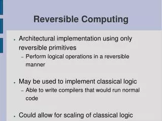
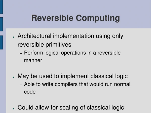
Reversible Computing • A reversible digital logic operation is: • Any operation that performs an invertible (one-to-one) transformation of the device’s local digital state space. • Or at least, of that subset of states that are actually used in a design. • Landauer’s principle only limits the energy dissipation of ordinary irreversible (many-to-one) logic operations. • Reversible logic operations can dissipate much less energy, • Since they can be implemented in a thermodynamically reversible way. • In 1973, Charles Bennett (IBM Research) showed how any desired computation can in fact be performed using only reversible operations (with basically no bit erasure). • This opened up the possibility of a vastly more energy-efficient alternative paradigm for digital computation. • After 30 years of (sporadic) research, this idea is finally approaching the realm of practical implementability… • Making it happen is the goal of the RevComp project at UF.
Adiabatic Circuits • Reversible logic can be implemented today using fairly ordinary voltage-coded CMOS VLSI circuits. • With a few changes to the logic-gate/circuit architecture. • We avoid dissipating most of the circuit node energy when switching, by transferring charges in a nearly adiabatic (literally, “without flow of heat”) fashion. • I.e., asymptotically thermodynamically reversible. • In the limit, as various low-level technology parameters are scaled. • There are many designs for purported “adiabatic” circuits in the literature, but most of them contain fatal flaws and are not truly adiabatic. • Many past designers are unaware of (or accidentally failed to meet) all the requirements for true thermodynamic reversibility.
Reversible and/or Adiabatic VLSI Chips Designed @ MIT, 1996-1999 By Frank and other then-students in the MIT Reversible Computing group,under CS/AI lab members Tom Knight and Norm Margolus.
AND Transition Tables • Recall how a truth table for Boolean logic lists all possible input combinations on the left, and the corresponding output(s) on the right. • A transition table is a similar device designed to allow us to easily distinguish reversible operations from irreversible ones. • We list each combination of all local bitsonce in both “before” and “after” columns. • Corresponding to just before the operation begins, and just after it is completely finished. • We draw an arrow from each before state to the particular after state that it transforms to. • Red if the transition is dissipative, green otherwise. • Must obey the following rule: Only one of the arrows going into any given after state may be green. • It is convenient to order the after column so thatall the green arrows go straight horizontally. • It may be that only a subset of the input and/or outputstates arise in the context of a given circuit design. • We may “fade away” the particular states and transitions which never arise. • An operation is always reversible iff there are no red arrows in the table. • This means the operation is one-to-one. • An operation is reversible in context iff there areno un-faded red arrows in the resulting table. • I.e., the operation is 1-1 on the states that arise. • We will find these tables to be very useful. Standard inverter(present-day “NOT gate”)operation. Function:out := ¬ in Usually irreversible. Only reversible in the context that itsinput never changes! cNOT (controlled-NOT) “gate” (operation) Function: D= C Always reversible.
Bistable Potential-Energy Wells A Technology-Independent Model of Digital Devices (Landauer ’61) • Consider any system having an (adjustable) potential energy surface (PES) in its configuration space. • The PES should have at least two local minima (or wells) • Therefore the system is bistable • It has two stable (or at least metastable) configurations • Located at well bottoms • The two stable states form a natural bit. • One state can represent 0, the other 1. • This picture can also be easily generalized tolarger numbers of stable states. • Consider now the PES havingtwo adjustable parameters: • (1) “Height” (energy) of the potential energy barrier between wells, relative to well bottoms • (2) Relative height of the left and rightstates in the well (call this “bias”) Potentialenergy 0 1 Generalizedconfigurationcoordinate
Possible Parameter Settings • In the following slides, we will distinguish six qualitatively different settings of the well parameters, as shown below… Raised BarrierHeight Lowered Left Neutral Right Direction of Bias Force
One Mechanical Implementation Boxspring Fixedsleevebearing Stateknob Gate rod Bias rod Rightwardbias Barrierwedge Leftwardbias Barrier up Barrier down
MOSFET Implementation • The logical state is in the location of a charge packet (excess of electrons) on either side terminal of a FET. • The charge packet might even consist of just a single excess electron in a sufficiently small (nanoscale) logic node. • The potential energy barrier is provided by the built-in voltage across the PN junctions in the FET. • The barrier height is lowered when the device is turned on by adjusting the voltage on the gate electrode. • Bias forces can be provided by (e.g.) capacitive coupling to nearby electrodes. n p n e e e
Possible Well Transitions (Ignoring superposition states.) • Catalog of all the possible transitions in the bistable wells, adiabatic & not... • We can characterize a wide variety of digitallogic and memory styles in terms of how theiroperation corresponds to subgraphs of this diagram. “1”states 1 1 1 leak 0 “0”states 0 leak 0 BarrierHeight ∆E k ln 2 ∆E N 1 0 Direction of Bias Force
Logic & Memory Styles All describable within the potential-well paradigm! • Irreversible styles: • Input-barrier, fixed-bias logic. • E.g. standard static CMOS inverters & combinational gates. • Input-bias, clocked-barrier latching. • Standard static CMOS latches, dynamic RAM cells, etc. • Reversible styles: • Type 1: Input-bias, clocked-barrier latching. • Type 2: Input-barrier, clocked-bias logic. • Type 3: Input-barrier, clocked-bias latching logic. • All of these are available in a very wide variety of different physical instantiations of the bistable well. • E.g., CMOS, superconducting, quantum-dot, Y-branch switches, mechanical implementations, etc.
Ordinary Irreversible Logics • Principle of operation: Lower a barrier, or not, based on input. Series/parallel combinations of barriers do logic. Major dissipation in at least one of the possible transitions. 1 Input changes, barrier lowered • Can amplify input signals. 0 Example: Ordinary CMOS logics Outputirreversiblychanged to 0 0
Irreversible SET/CLR operations SET operation • Irreversible SET: Turn on a pFET connecting node B to a high voltage source. B B Voltage color scheme: Low / High ½CV2 B • Irreversible CLR: Turn on an nFET connecting node B to a low voltage source. CLR operation B ½CV2 B B
Conventional Logic is Irreversible Even a simple NOT gate, as it’s traditionally implemented! • Here’s what all of today’s logic gates (including NOT) do continually, i.e., every time their input changes: • They overwrite previous output with a function of their input. • Performs many-to-one transformation of local digital state! • required to dissipate ≳kT on avg., by Landauer principle • Incurs ½CV2 energy dissipation when the output changes. Inverter transition table: Example: Static CMOS Inverter: in out
Example: Standard CMOS Inverter Inputgoeshigh Power (Vdd) Power (Vdd) on off In Out In Out = 0 = 0 = 1 = 1 Barrier btwn.Out and Groundlowered, charge“falls” to lowerenergy level off on Inputgoeslow Ground (0V) Ground (0V) Voltage color scheme: Low / High Barrierlowered Barrierraised Barrierlowered Simplified ← picture →of PES Charge falls in Charge falls out Vdd Vdd Out GND Out GND
Spacetime Logic Network Diagrams • In this general class of diagrams (popular in reversible & quantum logic), • Time is plotted in one direction, often left→right, • Horizontal lines denote locations (nodes, bits of state). • Operations (potential change events) are denoted by icons on and/or connections between bit-lines. • Please keep in mind: These diagrams do notdirectly depict the spatial structure of how a physical circuit is wired! • E.g., a long horizontal line denotes the evolution of a localized node in a physical circuit over a long period of time, not a long, spatially extended wire. • A vertical connection between lines or an icon on a line (often called a “gate”) denotes a momentary interaction event, not a perpetual physical link, or a physical object. An icon denotes that Opotentially changes (whetherspontaneously or under external control) at this time. This arrow denotes that some external event causes the value of node I to change at this time. I Location The change in I is propagated so as tocause node O to change a moment later. O Time
Inverter action in spacetime diagram • Note: This notation makes it explicit that an ordinary inverter’s real semantics is that it should carry out a logically irreversible transformation of its output node. Some outsideinfluence causesIn to possiblychange here In The “×” icon denotesthat the old valueof Out gets obliv-iously overwritten This (standard) icon denotesthat In’s value gets copied (with gain & delay) & invertedto produce the new Out. Location Out Time
Possible Well Transitions (Ignoring superposition states.) • Catalog of all the possible transitions in the bistable wells, adiabatic & not... • We can characterize a wide variety of digitallogic and memory styles in terms of how theiroperation corresponds to subgraphs of this diagram. “1”states 1 1 1 leak 0 “0”states 0 leak 0 BarrierHeight ∆E k ln 2 ∆E N 1 0 Direction of Bias Force
Ordinary Irreversible Memory • (1) Lower a barrier, obliviously erasing stored information.(2) Apply an input bias.(3) Raise the barrier to latch the new informationinto place.(4) Remove inputbias. (4) Retractinput 1 1 (1) and (2) can also be in theopposite order (4) Dissipationhere can bemade as low as kT ln 2 Retractinput 0 Barrierup 0 (3) Barrier up (3) (1) Examples:ordinaryDRAM cell,rod logicregister Input“1” Input“0” N 1 0 (2) (2)
Example: NMOS latch / DRAM cell Voltage color scheme: Low / Medium / High • Sequence corresponds exactly to general picture illustrated on previous slide. I M I M I M I M on off off off I M on I M I M I M I M on off off off (2) Apply inputbias (3)Raisebarrier (1) Obliviouserasure (4) Remove inputbias (& backto start) Could also do these in the other order also
Irreversible latch in spacetime diagram • Again, this notation makes it clear that irreversible behavior is occurring. I may changeagain later withoutnecessarilyaffecting value of M Outsideinfluence causesI to possiblychange here I Location The “×” & arrow denotes that the old value of M gets obliviously erased or overwritten by I when barrier islowered Later arrow denotes thatI gets reflected (without gain) inlocation M with a small delay M Barrier is raised shortlyafterwards (end of shaded area) Time
Conventional charging: Constant voltage source Energy dissipated: Ideal adiabatic charging: Constant current source Energy dissipated: Conventional vs. Adiabatic Charging For charging a capacitive load C through a voltage swing V Note: Adiabatic beats conventional by advantage factor A = t/2RC.
Adiabatic Switching with MOSFETs • Use a voltage ramp to approximate an ideal current source. • Switch conditionally,if MOSFET gate voltage Vg > V+VT during ramp. • Can discharge the load later using a similar ramp. • Either through the same path, or a different path.t≫RC t≪RC Exact formula:given speed fractions :RC/t Athas ’96, Tzartzanis ‘98
Requirements for True Adiabatic Logicin Voltage-coded, FET-based circuits • Avoid passing current through diodes. • Crossing the “diode drop” leads to irreducible dissipation. • Follow a “dry switching” discipline (in the relay lingo): • Never turn on a transistor when VDS≠ 0. • Never turn off a transistor when IDS ≠ 0. • Together these rules imply: • The logic design must be logically reversible • There is no way to erase information under these rules! • Transitions must be driven by a quasi-trapezoidal waveform • It must be generated resonantly, with high Q • Of course, leakage power must also be kept manageable. • Because of this, the optimal design point will not necessarily use the smallest devices that can ever be manufactured! • Since the smallest devices may have insoluble problems with leakage. Importantbut oftenneglected!
Possible Well Transitions (Ignoring superposition states.) • Catalog of all the possible transitions in the bistable wells, adiabatic & not... • We can characterize a wide variety of digitallogic and memory styles in terms of how theiroperation corresponds to subgraphs of this diagram. “1”states 1 1 1 leak 0 “0”states 0 leak 0 BarrierHeight ∆E k ln 2 ∆E N 1 0 Direction of Bias Force
Erasing Digital Entropy • Note that if the information in a bit-system is already entropy, • Then erasing it just moves this entropy to the surroundings. • This can be done with a thermodynamically reversible process, and does not necessarily increase total entropy! • However, if/when we take a bit that is known, and irrevocably commit ourselves to thereafter treating it as if it were unknown, • that is the true irreversible step, • and that is when the entropy iseffectively generated!! This state contains 1 bitof decomputable information, in a stable, “digital” form 1 This state contains 1 bitof physical entropy, but ina stable, “digital” form ? 1 0 0 Note: This transformation is reversible!! In these 3 states, there is noentropy in the digital state; it has all been pushed out into the environment. N 0
Reversible Set (rSET) & Clear (rCLR) • rSET operation semantics: Given assurance that a bit is initially 0,unconditionally change it to 1. • To implement: Traverse the adiabat (reversible trajectory) shown below. • Reverse this path to perform rCLR. (6) “1”states 1 1 Put workback in (1) “0”states 0 0 (5) Get workout BarrierHeight (2) (4) (3) N 1 0 Direction of Bias Force
Taking rSET & rCLR out of context • What happens if we attempt to perform rSET on a bit that is already a 1? • It still ends up with the right value (1), but… • Irreversible dissipation occurs in step 2 (when barrier is lowered), as shown below. • Similarly if we try to rCLR a 0. (1) (6) “1”states 1 1 1 (takeswork toraise 1) (takeswork toraise 1) “0”states (2) (5) (dissipatesit as heat) BarrierHeight (3) (4) N 1 0 Direction of Bias Force
rSET/rCLR transition tables • Note that these tables are not reversible according to the strict traditional definition… • Since they don’t represent a 1-1 transformation of all possible input states. • However, if we restrict our use of these operations so as to always avoid the input states that actually result in dissipation, • Then, we obtain a 1-1 transformation of the subset of the input states that are actually used, • And that is the correct statement of the true logical requirement for avoiding Landauer’s principle!
Type 1: Input-Bias Clocked-Barrier Reversible Latching (& Logic) (Can amplify/restore input signalin the barrier-raising step.) • Cycle of operation: • (1)Data input applies bias • Add forces to do majority logic • (2) Clock signal raises barrier • (3) Data input bias removed (3) 1 1 (4) Can reset latch reversibly (4) given copy ofcontents. (3) 0 0 (2) (4) (4) (4) (2) (1) (1) Examples:AdiabaticQCA, SCRL latch, Rod logic latch, PQ logic,Buckled logic, Helical logic N 1 0 (4) (4)
Type 1 Example: Adiabatic NMOS latch / DRAM cell • Same as irrev. latch, just skip the erasure step! Voltage color scheme: Low / Medium / High I M I M I M on off off I M on I M I M I M Can similarly use a CMOS transmissiongate (nFET/pFET pair) to latch a full-swing signal if necessary. on off off (1) Apply inputbias (2)Raisebarrier (3) Remove inputbias (Reverse stepsto reversiblyunlatch M)
P A Simple Reversible CMOS Latch • Uses a single standard CMOS transmission gate (T-gate). • Sequence of operation:(0) input level initially tied to latch ‘contents’ (output); (1) input changes gradually output follows closely; (2) latch closes, charge is stored dynamically (node floats); (3) afterwards, the input signal can be removed. Before Input Inputinput: arrived: removed:inoutinoutinout0 0 0 0 0 0 1 1 0 1 P in out • Later, we can reversibly “unlatch” the data with an exactly time-reversed sequence of steps. (0) (1) (2) (3) “Reversible latch”
Reversible latch in spacetime diagram I may be restored toneutral again later without necessarilyaffecting value of M Outsideinfluence causesI to possiblychange here I Location Arrow to dotted line denotes that changeto I is reversibly carried through (without gain) to location M at this time (energytransferred into I is also fanned out to M) Dotted lines denote that these nodes contain no informationat these times (they are ina predetermined state) M Barrier is raised some timeafterwards (end of shaded area) Barrier is lowered some timein here (start of shaded area) Time Note this operation is reversible only if I and Mmatch up exactly when they are first connected together! I Unlatchingsequence: M Time
Simplified Version of Diagram • Suppose the signal on the input node I was produced as a temporary copy of some origin node O. • We will see how to implement this reversibly later. • Then for simplicity of our diagrams, we may wish to omit explicit representation of the intermediate node I. • However, we must keep in mind that there is then a small additional space usage not explicitly shown in the diagram. O O “Reversible copy” I M M Time Time
Type 2: Input-Barrier, Clocked-Bias Reversible Retractile Logic • Barrier signal is amplified! Gain, restoring logic, fan-out. • Must reset output prior to changing input. • Combinational logic only! • Cycle of operation: • (1) Inputs raise or lower barriers • Do logic w. series/parallel barriers • (2) Clock applies bias force, which changes state, or not 0 0 0 (1) Input barrier height Examples:Hall’s logic,SCRL gates,Rod logic interlocks N 1 0 (2) Clocked bias force applied
Type 2 example: Adiabatic CMOS “buffer” (really, a cSET/cCLR gate) • Controlled-SET / controlled-CLEAR. • Structure: Essentially just a pair of CMOS transmission gates • 2 transistors each, an nFET and a pFET in parallel • Using dual-rail signaling, we can reversibly set or clear a bit on an unoccupied logic node (pair of voltage nodes), conditionally on an input node. • Amplifies input signal. • Fully restores logic levels. DriveN DriveN InN InN InP InP on on DriveN OutN OutN Voltage color scheme: Low / High DriveN DriveN InN off InN InN InP InP off off InP OutN OutN OutN (And similarly for OutP)
Spacetime diagram for buffer • Subscript NP notation denotes shorthand for dual-rail NP pair of wires. • Still denotes a single logical bit. • Diagram emphasizes that the buffer copies InNP’s value to a new location. • The value simultaneously remains available in the old location. • Dotted horizontal line shows that OutNP is empty prior to the operation. • The absence of “×” icon shows that the operation is reversible. • Buffer icon indicates that the input signal is being amplified and restored. • Note that the input comes from InNP, not from previous value of OutNP. • Downward wedges remind us the output remains dependent on the input. • Input can’t be changed without (possibly) irreversibly destroying output. • Fortunately, the buffer’s entire operation sequence is reversible! • So, sometime later on, we can unbuffer the output, • and then we are free to change the input. Input valuecan be changedafterwards. InNP InNP … OutNP Restored to null. OutNP Time Time
A This is our icon for a CMOS transmissiongate (T-gate). It saysthat nodes A and Bare connected wheneverthe control signal CNP has logic value 1. Reversible Buffered Latch CNP • Uses two dual-rail T-gates. • Combines a buffer and latch. • Reversibly copies InNP toMemNP when operated. B Spacetime diagram for operation sequence: InNP Physical structure: IntNP DriveNP MemNP InNP LatchNP Implements “reversible copy”: InNP MemNP IntNP MemNP