SS 2007
SS 2007. Geometrie in der Technik. H. Pottmann TU Wien. Kinematical Geometry. Overview. Kinematical Geometry Planar kinematics Quaternions Velocity field of a rigid body motion Helical motions Kinematic spaces. Planar Kinematical Geometry. Complex numbers and planar kinematics.


SS 2007
E N D
Presentation Transcript
SS 2007 Geometrie in der Technik H. PottmannTU Wien
Overview • Kinematical Geometry • Planar kinematics • Quaternions • Velocity field of a rigid body motion • Helical motions • Kinematic spaces
Complex numbers and planar kinematics • In the plane, a congruence transformation (x0,y0)(x,y), also called (discrete) motion, is given by x=a1+x0 cos-y0 sin, y=a2+x0 sin+y0 cos • Collecting coordinates in complex numbers z=x+iy, we get with a=a1+ia2, ei= cos+i sin • z=a+z0 ei, … rotational angle
Planar kinematics • a sequence of congruence transformations, depending continuously on a real parameter t, form a one-parameter motion • z(t)=a(t)+z0 ei(t) • For a point z0 in the moving system 0, z(t) describes its path (trajectory) in the fixed system
Example: trochoidal motion • Composition of two uniform rotations with angular velocities and , measured against the fixed system. • z(t) = aeit + z0eit ?
trochoids nephroid ellipse : = 1:-1 cycloid (composed of rotation and translation) cardioid: = 1:2 a=b
velocity field • velocity vectors are found by first derivative, • z‘(t)=a‘(t)+z0i‘(t)ei(t) • at a fixed time instant t=t0 we set ‘(t0)=: (angular velocity) and obtain a linear relation between points z and their velocity z‘: • z‘=a‘+i(z-a)
pole • For =0 we have an instantaneous translation • for≠0 we get exactly one point p with vanishing velocity, p=a+(i/)a‘ …. pole (expressed in the fixed system) • With p, the velocity field is z‘=i(z-p), i.e., the velocity field of a rotation about p… instantaneous rotation
polhodes • The locus of poles in the fixed (moving) system is called fixed (moving) polhode, respectively. • It can be shown that during the motion, the moving polhode rolls on the fixed polhode; the point of tangency being the instantaneous pole. z‘ z p
Trochoidal motion • polhodes are circles • Application of this motion in mechanical engineering (e.g. construction of gears)
Quaternion representation ofrotations • Discrete rotation about the origin, in matrix notation x=R.x0, R… orthogonal matrix • Orthogonality constraint on R, R.RT=I, is nonlinear. • A simplified representation, which is an extension of the use of complex numbers in planar kinematics, uses quaternions. This leads also to a parameterization of the set of orthogonal matrices.
quaternions • A quaternion is a generalized complex number of the form • q=q0+iq1+jq2+kq3 • The imaginary units i,j,k satisfy i2=j2=k2=-1 ij=-ji=k and cyclic permutations • H=R4 with addition and multiplication is a skew field
quaternions • conjugate quaternion q*=q0-iq1-jq2-kq3 (ab)*=b*a* • norm N(q)=q02+q12+q22+q32=qq* inverse q-1=q*/N(q)
Embedding R3 into H • We embed R3 into H as follows x=(x1,x2,x3) R3 x=ix1+jx2+kx3 • Now take a fixed quaternion a of norm 1 and study the mapping x‘=a*xa • We see: N(x‘) = x‘(x‘)*= a*xa a*x*a = = N(x)a*a = N(x)
Mapping x‘=a*xa • This mapping • is linear in x • preserves the norm • can be shown to have positive determinant • Therefore: x‘=a*xa represents a rotation about the origin • quaternion representation of rotations
Rotation with quaternions • From the quaternion a of norm 1, axis d (embedded in H) and angle of rotation follow by a=cos(/2)-d sin(/2) • The representation x‘=a*xa of a rotation yields a parameterization of orthogonal matrices R with help of the parameters a0,a1,a2,a3 (see lecture notes) • They satisfy a02+a12+a22+a32=1, and thus we have a mapping between rotations and points a on the unit sphere S3R4
applications • Examples for applications of the quaternion representation: • Design of motions (rotational part) via curve design in the 3-sphere S3 R4 • Shoemake: Bezier-like curves in S3 • Juettler and Wagner: rational curves in S3 • Wallner (2004): nonlinear subdivision in S3 • Explicit solution of the registration problem in R3 with known correspondences
First order instantaneous kinematics • One-parameter motion in Euclidean 3-space (not just rotation about origin) • Velocity vector fieldis linear: v(x) x x0(t) u(t) 0
derivation of velocity field • One-parameter motion x(t)=A(t).x0+a(t) • velocity field x‘(t)=A‘(t).x0+a‘(t) • express v(x)=x‘(t) in fixed frame by using x0=AT.(x-a) v(x)=A‘.AT.x+a‘-A‘.AT.a=:C.x+c
Derivation of velocity field • establish C as skew-symmetric by differentiation of the identity I=A.AT • 0=A‘.AT+A.A‘T=C+CT 0 -c3 c2 C= c3 0 -c1 -c2 c1 0 with c=(c1,c2,c3): C.x=cx
A c p x v(x) One-parameter motions with constant velocity vector field 1. translation 2. uniform rotation Rotation axis A has direction vector c and passes through points p with . ( … moment vector of the axis A)
One-parameter motions with constant velocity vector field • General case: helical motion • Helical motion is the composition of • a rotation about an axis A and • a proportional translation parallel to A A pt t p … pitch
Continuous (uniform) helical motion A spatial motion, composed of a einer uniform rotation abgout an axis a and a uniform translation parallel to a is called a uniform helical motion. a ... Helical axis h ... height Rotational angle and length of translation sproportional: a rotation with angle gedreht, so belongs to a translation of length s = p . The constant quotient p = s / is called pitch. f
Remark: discrete helical motion a • Any two congruent positions of a rigid body can be mapped into each other by a discrete helical motion. • It is composed of a rotation about an axis and a translation parallel to this axis. • In special cases two positions are related by a pure rotation or a pure translation.
Discrete and continuous case • In discrete case: • Any two positions can be moved into each other by a helical motion (or a special case of it) • In continuous case (consider two infinitesimally close positions) • The velocity field of a one-parameter motion at any time instant is that of a uniform helical motion (or a special case of it)
Axis and pitchof a helical motion • From the vector the axis and the pitchp of the underlying helical motion are calculated by: • a … direction vector of axis A • … moment vector of axis A [independent of the choice of q since qa = (q+a) a ] A a o q
Euclidean motion group embedded in the affin group • A Euclidean displacement x= a0+ A.x0= a0+x10a1+x20a2+x30a3 is a special affine map; A has to be orthogonal If A is an arbitrary matrix, we obtain an affine map. • Let us view an affine map as a point (a0,a1,a2,a3) in R12 (affine space)
a kinematic space • Associate a point in R12 with an affine copy of the moving body (affine map) • Euclidean (rigid body) motions are mapped to points of six-dimensional manifold M6 in R12 • Continuous motion is mapped to curve in M6 R12 A12
a(xi) R3 b(xi) Metric in R12via feature points (1) • Moving body represented by feature points X: x1, x2, … • Squared distance d2(a,b) between two affine maps and := sum of squared distances of corresponding feature point positions X
Metric in R12via feature points (2) • Euclidean metric in R12 which only depends on • barycenter • covariance matrix • Replace X by 6 verticesf1, …, f6 of inertia ellipsoid X a(fi) R3 b(fi)
Properties and facts • Sufficient to choose some points on the moving body and define the metric with the sum of squared distances of their positions (don‘t need an integral); in fact, sufficient to take vertices of the inertia ellipsoid • In the defined metric, the orthogonal projection of a point onto M6 can be computed explicitly (4th degree problem; use quaternions; see lecture on registration)
Curve approximation in robotics and animation • Interpolation or approximation of a set of positions by a smooth motion (Shoemake, Jüttler, Belta/Kumar,…) • Equivalent to curve interpolation/approximation in group of rigid body motion • Can use M6, S3,…
Problem formulation • Given N positions (ti) of a moving body at time instances ti, compute a smooth rigid body motion (t) which interpolates or approximates the given positions (t4) (t1) (t3) (t2)
A simple solution (1) • the given positions correspond to points in M6 • Interpolate them using a known curve design algorithm • results in affinely distorted copies of the moving body (called an affine motion) M6 R12
A simple solution (2) • Perform orthogonal projection of c onto M6 (i.e., best approximate each affine position by a congruent copy of the moving body; see registration with known correspondences) • The resulting curve c* is the kinematic image of the designed motion M6 R12 c* c
Energy minimizing motions • The following examples have been computed with an algorithm for the computation of energy minimizing splines in manifolds • This algorithm has been applied to compute an energy minimizing curve on M6R12. Thus, we obtain an energy-minimizing motion in R3
Motion smoothing • Curve smoothing on M6 yields motion smoothing