
DC Motor
E N D
Presentation Transcript
DC Motor • A simple model of a DC motor driving an inertial load shows the angular rate of the load, , as the output and applied voltage, , as the input. The ultimate goal of this example is to control the angular rate by varying the applied voltage. This picture shows a simple model of the DC motor.
A Simple Model of a DC Motor Driving an Inertial Load • In this model, the dynamics of the motor itself are idealized; for instance, the magnetic field is assumed to be constant. The resistance of the circuit is denoted by R and the self-inductance of the armature by L. • It is possible to develop differential equations that describe the behavior of this electromechanical system. In this example, the relationships between electric potential and mechanical force are Faraday's law of induction and Ampère's law for the force on a conductor moving through a magnetic field.
Mathematical Derivation • The torque seen at the shaft of the motor is proportional to the current i induced by the applied voltage. (t)=Km.i(t) where Km, the armature constant, is related to physical properties of the motor, such as magnetic field strength, the number of turns of wire around the conductor coil, and so on.
Motor equation The back (induced) electromotive force, vemf , is a voltage proportional to the angular rate seen at the shaft. Vemf (t) = Kb (t) where Kb, the emf constant, also depends on certain physical properties of the motor.
The mechanical part of the motor equations is derived using Newton's law, which states that the inertial load J times the derivative of angular rate equals the sum of all the torques about the motor shaft. The result is this equation,
A dc motor speed drive • The mathematical model of dc motor (permanent magnet type) can be expressed by these equations:
Dynamics of DC Motor • Typical dynamic responses are also shown. The motor is initially at standstill and at no load when a step command in speed is applied; when steady-state conditions are reached, a reversal of speed is commanded followed by a step load application.
The system is highly nonlinear due to the introduction of saturation needed to limit both the current delivered and the voltage applied to the motor. The system is in the saturation mode when the errors are large; as a consequence, the controller functions as a constant Current source, that is torque, resulting in the ramping of the speed since the load in this example is a pure inertia. The inclusion of saturation limits on the PI integrator is therefore necessary to provide antiwindup action. The presence of the signum function in the torque Expression is required in order to insure that the load is passive whether the speed is positive or negative (as is the case here).