Download

1 / 30
310 likes | 940 Vues
A secret history of the observed surface temperature record Phil Jones CRU, UEA. Developing the Global Temperature Record Terrestrial and Marine components Biases Boulder, June 2009. Earliest work – late 1970s and early 1980s.

E N D
A secret history of the observed surface temperature recordPhil Jones CRU, UEA Developing the Global Temperature Record Terrestrial and Marine components Biases Boulder, June 2009
Earliest work – late 1970s and early 1980s • Interpolation used inverse-distance weighted best fit planes with a base period of 1946-60 • The base period (i.e. using anomalies) is crucial in all the studies. It overcomes most elevation issues and some urbanization issues (later) • Grid points at 10° longitude by 5° latitude intersections • Station temperature data came from an NCAR DS, supplied on a 6250bpi tape • Assessed data for outliers and removed those beyond reasonable bounds • Programs ran on an IBM computer at Cambridge, for which cards had to be submitted • Assessment of the effects of sparser coverage in early decades • Compared results with all earlier studies • Jones, P.D., Wigley, T.M.L. and Kelly, P.M., 1982: Variations in surface air temperatures, Part 1: Northern Hemisphere, 1881-1980. Monthly Weather Review110, 59-70 • Kelly, P.M., Jones, P.D., Sear, C.B., Cherry, B.S.G. and Tavakol, R.K., 1982: Variations in surface air temperatures, Part 2: Arctic regions, 1881-1980. Monthly Weather Review110, 71-83 • Raper, S.C.B., Wigley, T.M.L., Mayes, P.R., Jones, P.D. and Salinger, M.J., 1984. Variations in surface air temperature. Part 3: The Antarctic, 1957-82. Monthly Weather Review112, 1341-1353
Pre-CRU land temperature series, each adjusted to have Brohan et al average (HadCRUT3) over their last 30 years of overlap (from Ch1 of AR4: zero line is 1961-90) AR4 shouldn’t have compared land only series with HadCRUT3!
Mid -1980s • Extended the spatial coverage of the station record, by digitizing records held in Met Office and other archives • Assessed homogeneity of the records (subjectively) • Base period of 1951-70 • Each station associated with its nearest grid point (as in 1982) and weights were inverse distance • More extended analysis of the effects of fewer stations in the early decades (using frozen grids) • Record extended back to 1851 (from 1881 earlier) • First combined land and marine temperature record in 1986 • Jones, P.D., Raper, S.C.B., Bradley, R.S., Diaz, H.F., Kelly, P.M. and Wigley, T.M.L., 1986: Northern Hemisphere surface air temperature variations: 1851-1984. Journal of Climate and Applied Meteorology25, 161-179 • Jones, P.D., Raper, S.C.B. and Wigley, T.M.L., 1986: Southern Hemisphere surface air temperature variations: 1851-1984. Journal of Climate and Applied Meteorology25, 1213-1230 • Jones, P.D., Wigley, T.M.L. and Wright, P.B., 1986: Global temperature variations, 1861-1984. Nature322, 430-434
Comparison of the versions across the years(1982, 1986, 1994, 2003 and 2006) NH – Top SH – Bottom Left – as was Right – 1951-80 Q – was all the effort worth it? It shows how robust the series is!
Questions that began to be asked (1)(some despite being discussed the papers) • Effect of sparser coverage – don’t you need more stations? • The frozen grid analyses had effectively answered this, but many only became convinced once the uncertainties were displayed with error ranges • These also led to the understanding of the number of spatial degrees of freedom (Neff) • Looking at numerous seasonal and annual temperature anomaly maps indicated that Neff must be much smaller than the number of observing sites, and that the number varies depending on the season and on the timescale • The paper that derived the necessary formulae (Jones et al., 1997) was based on the Wigley et al. (1984) r-bar paper • The fact that Neff was about 100 led to the cottage industry of reconstruction the past temperatures from natural and documentary proxies • The fact that r-bar is higher in winter implies that these would be much better, if we had more winter-responding proxies • Wigley, T.M.L., Briffa, K.R. and Jones, P.D., 1984: On the average value of correlated time series with applications in dendroclimatology and hydrometeorology. Journal of Climate and Applied Meteorology23, 201-213 • Jones, P.D., Osborn, T.J. and Briffa, K.R., 1997: Estimating sampling errors in large-scale temperature averages. J. Climate10, 2548-2568
Questions that began to be asked (2) • Isn’t the fact that most sites have moved more than once in their history important? • We’d addressed the long-term homogeneity of the station series in the mid-1980s • The effort was large in person years, but it’s affect was barely noticeable (the comparison of the 1982 and 1986 papers showed this) • Clearly important for individual series, but not that vital as the space scale increases
Homogenisation adjustment uncertainty Black line is based on 763 sets of adjustments Red – hypothesised distribution Blue – the difference, so that used for stations where adjustments have not been made
Similar bimodal distribution in a recent paper on the USHCN Menne et al (2009) in BAMS
USHCN – all and 70 best (latter partly determined by surface stations.org) The 70 obviously omit large parts of the contiguous US
Questions that began to be asked (3) • Isn’t the world warming because of many stations being located in cities? • The urbanization issue! People always remember the greatest UHI that someone has shown on a particular day! • They forget the similar warming between the land and the ocean components • Comparisons of rural-only station datasets • One new example here (London) • Recognition that UHIs exist, but what matters is urban-related warming trends not the UHI size • Jones, P.D., Groisman, P.Ya., Coughlan, M., Plummer, N., Wang, W-C. and Karl, T.R., 1990: Assessment of urbanization effects in time series of surface air temperature over land. Nature347, 169-172 • Jones, P.D., Lister, D.H. and Li, Q., 2008: Urbanization effects in large-scale temperature records, with an emphasis on China. J. Geophys. Res. 113, D16122, doi:10.1029/2008/JD009916.
Urbanization Influence • Homogeneity testing may not remove all urban affected sites if all sites are similarly affected by urban growth • Approach to assess residual effect is to develop a dataset of rural-only stations. • Grid the rural-only stations and then compare with the grid with all the stations • The issue here is assessment of the effect on monthly and annual average temperatures – not the effect on a single day
Urbanization Examples • Few studies have looked at urbanization studies across large areas of the world • Major studies are Jones et al. (1990), Parker (2004, 2006) and Peterson and Owen (2005) – references in Chapter 3 of AR4 • Basic conclusion is that any residual warming is an order of magnitude less than the warming that has occurred over the last 100 years • Effect can be large in rapidly developing areas like China – but even here the large-scale warming is 1.6 times greater (Jones et al. 2008).
London UHI greater for Tn than Tx. Central London sites always warmest at night, but warmer during day west of London London has an Urban Heat Island (UHI), but no urban-related warming since at least 1900. In other words, the centre got warmer earlier.
Questions that began to be asked (4) • What causes the temperatures to change so much from year to year? • El Niño and La Niña (ENSO) explain some of the high-frequency variability • Volcanoes cause cooling • Circulation change can cause warming and cooling (e.g. COWL patterns) • Possible to factor out these influences • Jones, P.D., 1989: The influence of ENSO on global temperatures. Climate Monitor 17, 80-89 • Thompson. D.W.J., Wallace, J.M., Jones, P.D. and Kennedy, J.J., 2009: Removing the signatures of known climate variability from global-mean surface temperature: Methodology and Insights. J. Climate (tentatively accepted).
Questions that began to be asked (5) • There are sites moves and/or urbanization influences at the nearby site (to where this talk is being given) • You’ve very few sites in Africa and South America • Few seem to follow the logic of the Neff argument and think that one site can influence the global average • Seem to accept the limited number when it comes to proxy data, but not when it is instrumental data ! • Developing these series (or regional ones) brings so many insights, which are clearly apparent in examples • Different observation times (and methods of calculating mean T) in different countries don’t matter, as long as they don’t get changed • A few outliers don’t matter. I once had some 100°C anomalies for a few boxes in Siberia, but the effect on NH averages was a few hundredths • Combining the wrong month’s station data with a different month’s absolute temperatures produces far greater differences (as GISS realised last year!)
Issues Today • SST measurement • Exposure of thermometers in Europe in summer in the mid-19th century • Homogeneity of daily temperature series – easiest to use the monthly adjusted series, and change the daily accordingly (not addressed here)
What does the corrected series look like? HadSST2 (no corrections after 1941) HadSST2 (no corrections after 1941) Global-average SST anomaly (°C) wrt 1961-1990 Uncorrected data Uncorrected data
Other Marine (SST) problems • The various measuring platforms (ships, buoys, satellites etc) have slightly different biases • SSTs in the 1940s (Thompson et al., 2008) • Recent SSTs (buoys slightly cooler than ships) • Neither of these two adjusted for yet • Issue is the same in all cases – instruments improved (response time, better sampling etc.) but no overlap measurements made beforehand. The bias gets sorted out in retrospect, when there is enough data available to clearly show the problem • Thompson, D.W.J., Kennedy, J.J., Wallace, J.M. and Jones, P.D., 2008: A large discontinuity in the mid-twentieth century in observed global-mean surface temperature. Nature453, 646-649.
Huge change in marine observing network in the past 25 years Percentage of observations coming from DRIFTERS and SHIPS
What will the corrected series look like? New Corrections HadSST2 (no corrections after 1941) Global-average SST anomaly (°C) wrt 1961-1990 Uncorrected data
Early exposure issues • Europe affected, before the development of Stevenson screens • Solution has come about from modern parallel measurements (in Austria and Spain, with the old screens) • Effect is annually ~0.4°C, with most series too warm by up to 0.7°C in June • Surprisingly (for Austria), the effect is much smaller using the (Tx+Tn)/2 method of calculating averages than using fixed hours • Issue important as it is the summers that calibrate the natural and documentary proxies
Kremsmünster - Austria When built in the 1770s, this monastery was the tallest in Europe for the time
Kremsmünster – historic minus modern diurnal cyclesNNE exposure Work undertaken by Reinhard Böhm et al (ZAMG, accepted Climatic Change) 8 complete years of overlap between the ‘window’ and the modern Austrian observing site
Effect through different formulae used to calculate monthly mean T
Adjustment across all 32 sites in the Greater Alpine Region (GAR) GAR is 4-19°E by 43-49°N To apply adjustments need to know the NW-to-NE direction each site faced
Effect of changes across the GAR Thin is raw data. Grey is after adjustment for site moves and observation time changes. Thick shows the effect of exposure issues (thick black overlies grey since about 1860).
Conclusions • Individual station homogeneity assessment has little effect on global averages, but is vital for local- and regional-scale homogeneity • Biases (buckets and some urbanization) are what is important for homogeneity (particularly the way SSTs have been measured) • Problems in the 1945-55 will be adjusted for as well as issues of the differences between ships and drifters today (Effect will to delay the post-WW2 cooling to the mid-1950s and will slightly raise temperatures over the last 10 years) • Exposure issues with pre-screen measurements addressed in Europe (Effect is to cool summer temperatures by about 0.5°C before about 1860) • 2001-2008 0.18°C warmer than 1991-2000, which was 0.14°C warmer than 1981-90