Download
1 / 21
210 likes | 296 Vues
Sea-Level Change Driven by Recent Cryospheric and Hydrological Mass Flux. Mark Tamisiea Harvard-Smithsonian Center for Astrophysics. Thanks to:. Extracting Source Information From Geographic Sea Level Variations. Introduction Terminology Physics

E N D
Sea-Level Change Driven by Recent Cryospheric and Hydrological Mass Flux Mark Tamisiea Harvard-Smithsonian Center for Astrophysics Thanks to:
Extracting Source InformationFrom Geographic Sea Level Variations • Introduction • Terminology • Physics • Patterns for Greenland, Antarctica and glaciers • Obtaining Greenland and Antarctic Ice Mass Balance • Select set of tide gauges • Binning of many tide gauges • Future Directions • Improvements to fingerprints • Focus on near field • New data types • Geoid better discriminator? • Integration with ocean modeling • Large oceanic variability • Hydrological example
IntroductionSea Level Variations Due to Loads References: • Farrell and Clark [1976] • Clark and Primus [1987] • Nakiboglu and Lambeck [1991] • Conrad and Hager [1997] • Mitrovica et al. [2001] • Plag and Jüttner [2001] • Assumptions: • Static Ocean Response • Elastic Earth (generally) Load Ocean • Possible Loads: • Ice Sheets • Glaciers • Water Stored on the Continents
Load Changes • More water in ocean • Crust and sea surface adjust to the changing mass load Ice sheet melts -- or -- River basin loses water
Uniform Melting Meier, 1984 Melting Scenarios
RSL Fingerprints from Melting Ice Sheets and Glaciers Antarctica Greenland Mountain Glaciers 1.0 corresponds to value of globally-averaged sea level rise.
Obtaining Greenland and Antarctic Ice Mass Balance Adding up the Contributions ΔRSL (at a given point) = Contributions from Glacial Isostatic Adjustment (GIA)+ Antarctica + Greenland + Glaciers + Steric Effects + Atmospheric Effects + Currents + Hydrology + Tectonics + Sedimentary Loads + … Assume large spatial scales and long time scales leave only a few contributions.
First Example: Small Number of Tide Gauges Mitrovica et al., 2001 Tamisiea et al., 2001
Select Set of Tide Gauges Douglas, 1997
Raw Tide Gauge Data GIA Corrected Tide Gauge Data
Second Example: Binning of Many Tide Gauges Plag, 2006. • Tide gauge data binned • Numerous regression estimates generated by varying binning resolution, GIA model, and steric model Results: Antarctic Contribution: 0.4 ± 0.2 mm/yr Greenland Contribution: 0.10 ± 0.05 mm/yr Global Average: 1.05 ± 0.75 mm/yr 10 to 15% Variance Reduction Also, see poster by C.-Y. Kuo and C.K. Shum
Future Directions • Improvements to fingerprints • Focus on near field • New data types • Geoid better discriminator? • Integration with ocean modeling • Large oceanic variability • Hydrological example
1. Fingerprint Improvements Uniform Melting Mass balance scenario adapted by James and Ivins, 1997 from Jacobs, 1992. Tamisiea et al., 2001
2. Focus on Near Field • The impact of different melting scenarios greatest in near field. • Saltmarsh proxy records with uncertainties of 0.25 mm/yr would still resolve difference in models to the right. Milne and Long
Alaska – Earth Model Dependence Glacier model based on Arendt et al., Science, 2002 mm/yr
Effects of Earth Model on Sea Surface and RSL Tamisiea et al., 2003
3. Integration with Ocean Modeling • Interannual variability large • Incorporate fingerprinting technique into models to perform integrated analysis Altimeter MIT/AER ECCO-GODAE solution range (0-10 cm) Source: Ponte et al.
Comparison of Tide Gauge Time Series with Ocean Model Hill, Ponte, and Davis, 2006 A combined time series including Inverted barometer time series [Ponte, 2006] Ocean model time series [courtesy of D. Stammer] were compared to the time series of 380 globally-distributed PSMSL tide gauges While removing the model time series significantly reduces the mean global variance, an annual signals remains. [Figure removed] Example time series for stations with high variance reduction (red=tide gauge, blue=model)
Example: Annual SignalLaDWorld Hydrology Dataset [Figure removed] Milly and Shmakin, 2002 Milly, Cazenave, and Gennero, 2003 • Long time series • Predicted GMSL close to observed
Variance Reduction of Tide Gauge Data [Figure removed] • Hydrology model time series removed from residual time series (TG-OM-IB) • Variance reduced
Conclusions • Fingerprinting offers another method of constraining the sources of sea level rise. • Large regional effects could provide more effective test of regional mass variation scenarios. • Inclusion into dynamic ocean models should improve the ability to recover these static signals from the tide gauge and altimetry data.