Understanding Sea Level Change: Concepts, Factors, and Historical Developments
This chapter provides a comprehensive overview of sea level change (SLC), focusing on fundamental definitions, contributing factors, and historical developments per the IPCC reports. Topics include the significance of relative sea level measurements, the influences of ocean heat expansion and land-ice melt, and advancements in modeling approaches, including coupled models that enhance projections. The chapter also highlights the increasing rate of sea level rise in the 21st century and emphasizes ongoing uncertainties in regional projections and ice sheet contributions, underscoring the complex nature of SLC dynamics.

Understanding Sea Level Change: Concepts, Factors, and Historical Developments
E N D
Presentation Transcript
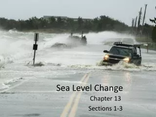
Sea Level Change Chapter 13 Sections 1-3
Agenda: • Fundamental Definitions and Concepts • Primary contributing factors to SLC • Developments through time of the IPCC report • Processes Affecting SLC • Models • Historical Geological Periods and their climates • GMSLC in the past 100 years
Fundamental Definitions and Concepts • Relative Sea Level (RSL): the height of the ocean surface at any given location with respect to the surface solid of the earth • RSL is more relevant for considering the coastal impacts of SLC • Measured over longer time spans from geological records 13.1
Fundamental Definitions and Concepts • Geocentric Sea Level: reference ellipsoid • Measured over the past 20 years using satellite altimetry 13.1
Fundamental Definitions and Concepts • Mean Sea Level (MSL) • temporal average for a given location, this gets applied to remove shorter period variability • The use of the word “sea level” in chapter 13 is MSL • Global Mean Sea Level • when you average MSL spatially • Change in ocean water volume • Integrating RSL change over ocean area • This volume is directly related to the processes that dominate SLC (changes in ocean temperature and land-ice volume) 13.1
Primary contributing factors to SLC • expansion of the ocean as it warms • Observations show that the largest increase in the storage of heat in the climate system has been in the oceans • transfer of water as it is currently stored on land, particularly from land ice (glaciers and ice sheets) 13.1
Developments through time of the IPCC report • First IPCC Report (FAR) lays groundwork for our current understanding • Sea level has risen in the 20th century • The rate of rise has increased when compared to the 19th century • Ocean thermal expansion and mass loss from glaciers were the main contributors to 20th century SLC • The rate of rise in the 21st century is predicted to surpass that of the 20th century • Sea level will not raise uniformly around the world • Sea level will continue to rise well after GHG emissions are reduced 13.1
Developments through time of the IPCC report • Third Annual Report (TAR) • Introduces the coupled Atmosphere-Ocean General Circulation Models (AOGCM’s) and ice sheet models to replace energy balance climate models as the primary way to project SLC • Allows us to consider regional distribution of SLC in addition to the global average 13.1
Developments through time of the IPCC report • Fourth Annual Report (AR4) • Existing Ice sheet models can’t simulate recent observations of accelerations • Our understanding of ice sheet dynamics is too limited to assess the likelihood of future accelerations or to provide an estimate of the upper bound that the future may bring 13.1
Developments through time of the IPCC report • Remaining Issues: • Observed SLC over decades is actually larger than the individual contributions estimated by our models • Confident projections are not possible on the regional distribution of sea level rise • Insufficient understanding of the potential contributions from ice sheets 13.1
Numbers through time in the ARs Numbers in the Annual Reports: FAR: 31 to 110 cm SAR: 13 to 94 cm TAR: 9 to 88 cm AR4: 18 to 59 cm 13.1
Oceans • changes in currents, ocean density, and sea level are all tightly coupled • changes in one location impact local sea level and sea level far from the location of the original change • This includes coastal SLC • Only temperature change produces a significant contribution to global average ocean volume change because of thermal expansion and contraction • Overall, these processes cause sea level to vary on a broad range of spatial and temporal scales (from short lived events to changes over several decades) 13.1
Water and Ice Mass Exchange • exchange of water between land and the oceans leads to a change in GMSL • This is a signal that propagates rapidly throughout the globe • all regions experience SLC within days of the mass being added • An influx of freshwater changes ocean temperature and salinity, thus impacting currents and local sea level 13.1
Sediment Transfer from the Coastal Zone • particularly important in deltaic regions • these can dominate the SLC in these localized areas but are less important on a regional/global scale • estuaries contribute 0.01 mm / year 13.1
Models Used to Interpret Past, and project future SLC • Atmospheric Oceanic Global Circulation Models: • have components that represent the ocean, atmosphere, land, cryosphere, and simulate sea surface height changes resulting both from natural forcing (volcanoes) and GHG increases • also exhibit internally generated climate variability: ENSO, Pacific Decadal Oscillation, North Atlantic Oscillation • critical components for global and regional change: surface wind stress, air-sea heat and freshwater flux 13.1
Models Used to Interpret Past, and project future SLC • Geodynamic surface-loading models: • simulate the RSL response to past and contemporary changes in surface water and land-ice mass redistribution, and contemporary atmospheric pressure changes • They do not consider Ocean dynamics • Instead they focus on annual variability driven by contemporary changes in the hydrological cycle 13.1
Storm surge and wave-projection models • used to assess how changes in storminess and MSL impact sea level extremes and wave climates • dynamical models • statistical models • SEM 13.1
Semi-Empirical Models (SEM’s) • Classification of models • project sea level based on statistical relationships between observed global mean sea level and global mean temperature • parameters are determined from observational data • they don’t simulate the underlaying properties 13.1
Process-based models: • (classification of models) • sea level and land ice models that simulate the underlying processes 13.1
Models for projecting changes in Ice Sheets • AOGCMs • Modeling glaciers and ice sheets is not yet at a stage where projections of their changing mass are routinely available • Process-based models can use outputs of AOGCMs to project the affects of climate change on ice masses 13.1
Models for projecting changes in Ice Sheets • Surface Mass Balance (SMB) • this is the overall contribution of an ice mass to the sea level • caused by changes in the dynamics that affect outflow (i.e. solid ice discharge) to the ocean 13.1
Models for projecting changes in Ice Sheets • Projecting the sea level contribution of land ice • compare the model results with a base state assuming no sea level contribution • this base is taken from the pre industrial period 13.1
Models for projecting changes in Ice Sheets • Regional Climate Models (RCMs) • incorporate sophisticated representations of mass and energy budgets associated with snow and ice surfaces • These are the primary sources of the SMB projections • Success of this modeling approach relies on the computational grid to evolve to continuously track the migrating calving front • This is challenging because typical computational grids on three dimensional models of ice sheets are fixed in space 13.1
Models for projecting changes in Ice Sheets • Problems: Small number of glaciers with mass budget info available • this is the main challenge for modelers • stats techniques can be used to derive relationships between SMB ad climate variables for the small sample that has been surveyed • then these can be upscaled to the other regions of the world 13.1
SLC in the past • Examining past records of SLC in order to gain insight into the sensitivity of sea level to PAST climate change • Using this as a record to understanding current climate change • Helping us understand the amplitude and variability during past periods when climate was warmer than pre-industrial • Helps us better account for uncertainties 13.2
Middle Pliocene • The Pliocene is the time period 5.3 million to 2.6 million years ago • Global Climate average is 2-3 degrees C higher than today • Extensive glaciation occurs over Greenland in the Late Pliocene 13.2
Middle Pliocene • Med. confidence: GMST 2-3.5 degrees C warmer versus pre-undustrial climate • GMSL was higher than today, low agreement on how high 13.2
Marine Isotope Stage 11 • Interglacial Period between 424,000 and 374,000 years ago • comparable GHG concentrations to the pre industrial age • Most paleoclimate observations come from this time period • This is the best geological analogue for the natural development of climate in the holocene and future climate • We compare the current interglacial period (Holocene) with previous warm periods, like this one 13.2
Marine Isotope Stage 11 • Temperature in MIS11 • 1.4 to 2.0 degrees C warmer than pre-industrial based on Antarctic ice core (low confidence) • GMSL • 6 to 15 m higher than present (med. confidence) • Requires a lot of or most of the present day Greenland Ice sheet • Evidence from beach deposits in Bermuda and the Bahamas 13.2
Late Holocene • Holocene begins 11,000 years ago • Improved understanding of SLC in the past 7,000 years since AR4 • from 7 to 10,000 years, GMSL probably rose from 2 to 3 meters, to near present levels • Based on local sea level records from the past 2000 years, there is med. confidence that changes in GMSL have not exceeded + or - 0.25 meters on time scales of ~100 years 13.2
Late Holocene • The most robust measure comes from salt marshes • This supports the AR4 conclusion of low rates of GMSL change from the late holocene to modern times • Gehrels and Woodworth (2013) argue that SLC begins in the late Holocene, between 1905 and 1945 13.2
The Instrumental Record (1700-2012) • Tide Gauges • Composed of tide gauges over the past 2-300 years • Some of the first gauges were installed in European ports in the 1700s • Southern hemisphere measurements only started in the late 1800s • Satellites • since the early 1990s: satellite based radar altimeter measurements • The satellite record is high precision and it provides measurements at 10 day intervals • There is very good agreement on the 20 year long GMSL trend 13.2
Paleo sea level data for the last 3000 years from Northern and Southern Hemisphere sites. The effects of glacial isostatic adjustment (GIA) have been removed from these records. Light green = Iceland (Gehrels et al., 2006) purple = Nova Scotia (Gehrels et al., 2005), bright blue = Connecticut (Donnelly et al., 2004), blue = Nova Scotia (Gehrels et al., 2005), red = United Kingdom (Gehrels et al., 2011), green = North Carolina (Kemp et al., 2011), brown = New Zealand (Gehrels et al., 2008), grey = mid-Pacific Ocean (Woodroffe et al., 2012).
Sea Level Data from salt marshes since 1700 From Northern and Southern Hemisphere sites compared to sea level reconstruction from tide gauges (blue time series with uncertainty) (Jevrejeva et al., 2008) Ordinate axis on the left corresponds to the paleo sea level data. Ordinate axis on the right corresponds to tide gauge data. 13.2
GMSL constructed from tide gauges from three different approaches Orange from Church and White (2011), blue from Jevrejeva et al. (2008), green from Ray and Douglas (2011) (see Section 3.7). 13.2
Altimetry Data from 5 groups (University of Colorado (CU), National Oceanic and Atmospheric Administration (NOAA), Goddard Space Flight Centre (GSFC), Archiving, Validation and Interpretation of Satellite Oceanographic (AVISO), Commonwealth Scientific and Industrial Research Organisation (CSIRO)) with mean of the five shown as bright blue line (see Section 3.7). 13.2
Major Points 13.2 • it is likely that the rate of sea level rise is increased from the 19th century to the 20th century • high confidence that the rate of SLR has increased during the last 200 years • it is likely that GSML has accelerated since the early 1900s 13.2
Major contributions to GMSL in the instrumental age • Chapter focus: • comparing observed to modeled, and seeing if they match • a major advance in what we are able to observe is through the Argo Project’s global coverage, as well as ship based data of the open ocean • Modeling: • GMSL in the last Instrumental period is proportional to the increase in ocean heat content • Historical GMSL rise due to thermal expansion is simulated by CMIP5 below • There is high confidence in projecting thermal expansion using AOGCMs 13.3
Ocean Thermal Expansion • Individual CMIP5 Atmosphere–Ocean General Circulation Model (AOGCM) simulations are shown in grey • the AOGCM mean is in black • observations in teal with the 5 to 95% uncertainties shaded. 13.2 13.3
Glaciers • all land ice masses including those peripheral to but not including the Greenland and Antarctic ice sheets • The earliest sea level assessments recognize glaciers as a significant contributor to GMSL rise (Meier 1984) • compare simulations to the Gravity Recovery and Climate Experiment data (GRACE), as well as satellites • there is now a complete inventory as well 13.2 13.3
Glaciers • combined records indicate a net decline in global glacier volume beginning in the 19th century • It is likely that anthropogenic forcing played a statistically significant role in accelerating global glacier loss in the later decades of the 20th century vs. rates in the 19th century • from 2003-2009, glaciers contributed .71 mm per year 13.2 13.3
Glacier models There is medium confidence in the use of glacier models to predict global projections based on AOGCMs • Model simulations by Marzeion et al. (2012a) with input from individual AOGCMs are shown in grey with the average of these results in bright purple. • Model simulations by Marzeion et al. (2012a) forced by observed climate are shown in light blue. • The observational estimates by Cogley (2009b) are shown in green (dashed) • Leclercq et al. (2011) in red (dashed).
Greenland and Antarctic Ice Sheets • Contribution of GMSL rise: • Greenland: very likely has increased from 0.09 to 0.59 mm / yr from 2002-2011 • Antarctica: likely increased from 0.09 to 0.40 for 2002-2011. 13.2 13.3
Rate of change for ice sheets 13.2 13.3
Key takeaways • From 1993-2010, allowing for uncertainty, GMSL rise is consistent with the sum of observed estimates • The biggest contributors are ocean thermal expansion (35% of the GMSL rise) • glacier mass loss (25% of GMSL rise (doesn’t include Greenland and Antarctica) • Observations show an increased contribution from ice sheets over the past 20 years 13.2 13.3