Cost Benefit Analysis Evaluation Techniques
Cost Benefit Analysis Evaluation Techniques. Social Discount Rate. Discounting rooted in consumer preference We tend to prefer current, rather than future, consumption Marginal rate of time preference (MRTP) Face opportunity cost (of foregone interest) when we spend not save

Cost Benefit Analysis Evaluation Techniques
E N D
Presentation Transcript
Cost Benefit Analysis Evaluation Techniques
Social Discount Rate • Discounting rooted in consumer preference • We tend to prefer current, rather than future, consumption • Marginal rate of time preference (MRTP) • Face opportunity cost (of foregone interest) when we spend not save • Marginal rate of investment return
Intergenerational effects • We have tended to discuss only short term investment analyses (e.g. 5 yrs) • What about effects in distant future? • Called intergenerational effects • Economists agree that discounting should be done for public projects • Do not agree on positive discount rate
An example • Someone offers you choice of $1000 now and $1200 in one year • If you have no preference (indifferent) then your MRTP is 20%
Discounting handout • How much do/should we care about people born after we die? • Higher the discount rate, the less future values will count compared to today • Ethically, no one’s interests should count more than another’s • Implies there is no justification for discounting across long time periods • Called ‘equal standing’
Climate Change • Discussions ongoing about how best to manage global CO2 emissions to limit effects of global change • Should we sacrifice short-run economic growth to do something to improve environment and leave resources for the future? • Really asking 2 separate questions!
Two Questions • What duty do we have to make sacrifices for future generations? • If we sacrifice, what is the optimal policy to maximize benefit? • So we should compare global change proposals with alternatives • Perhaps higher R&D spending on science or medicing would have higher benefits!
Some evidence • Cropper et al surveyed 3000 homes • Asked about saving lives in the future • Found a 4% discount rate for lives 100 years per now • Equal standing does not imply different generations have equal claims to present resources! • Harsanyi says only do so if their marginal gain is higher than our loss
More evidence • If future generations will be better off than us anyway • Then we might have no reason to make additional sacrifices • There might be ‘special standing’ in addition to ‘equal standing’ • Immediate relatives vs. distant relatives • Different discount rates over time • Why do we care so much about future and ignore some present needs (poverty)
Types of Valuation • Valuations can be put on either stocks or flows • Use Value • Non-Use Value • Option Value
Sources of economic value USE VALUES NON USE VALUES OPTION VALUE Benefits that derive from the actual use of the natural resources. • Those benefits which do not imply a contact between the consumers and the good.Non-use values are also called "existence value". The arguments behind existence value are: • Intrinsic value • Bequest motive Value placed on environmental assets by those people who may want to secure the use of the good or service in the future. Option values can be either positive or negative.
Example of Total economic value The analyst should be sure that the values to be counted are not mutually exclusive or that they are not already captured by other value components.
Methodological approaches REVEALED PREFERENCES (Observed Behavior) STATED PREFERENCES(Hypothetical) The analyst uses actual behaviour to recover the consumer’s preferences, and then uses this information to work out money measures of the consumer’s welfare changes. The analyst uses information that is based on what the consumer states when directly asked to express his value judgement.
Methods REVEALED PREFERENCES (Observed Behavior) STATED PREFERENCES(Hypothetical) • Direct • Market Price • Simulated Markets • Indirect • Travel Cost • Hedonic Property Values • Hedonic Wage Values • Avoidance Expenditures • Direct • Contingent Valuation • Indirect • Contingent Ranking
Direct Revealed Preference • Examples • Medical costs for increased Asthma treatment due to air pollution • Lost income to fishermen, from oil spill. • Issues • Scientific uncertainty • Example: identifying relationship between pollution and health (without being able to do controlled experiments).
Indirect Revealed Preference • Cannot directly observe the cost of pollution • Might be able to infer those costs, from market behavior • Avoidance Expenditures • Hedonic Property Values • Hedonic Wage Values • Travel Cost
Avoidance • Groundwater contaminated in Pennsylvania • Residents informed: 3 possible responses • Bottled Water • Boiling Water • Home Water Treatment System • Economists tracked the avoidance expenditures & costs (including opportunity costs) to get an estimate of economic damages.
Hedonics and Travel Cost • Travel Cost Model: use data from actual visitations, estimate cost of travel, derive demand curve for visits to the “site”. • Hedonic Price Method: compare products with similar attributes but one “bundles” an environmental good. • Derive demand for the environmental good. • House prices influenced by environmental amenity (e.g. noise) • Wages influenced by riskiness of job
Why Use Travel Cost? • Site is primarily valuable to people as a recreational site. There are no endangered species or other highly unique qualities that would make non-use values for the site significant. • The expenditures for projects to protect the site are relatively low. Thus, using a relatively inexpensive method like travel cost makes the most sense. • Relatively simple compared to other methods
Why Use Travel Cost? • Time is a valuable commodity (time is $) • Most major transportation/infrastructure projects built to ‘save travel costs’ • Need to tradeoff project costs with benefits • Ex: new highway that shortens commutes • Differences between ‘travel’ and ‘waiting’ • Waiting time disutility might be orders of magnitude higher than just ‘travel disutility’ • Why? Travelling itself might be fun
Travel Cost Method • Basic premise - time and travel cost expenses incurred to visit a site represent the “price” of access to the site. • Thus, peoples’ WTP to visit the site can be estimated based on the number of trips that they make at different travel costs. • This is analogous to estimating peoples’ WTP for a marketed good based on the quantity demanded at different prices.
Travel Cost Model • Goal: To derive demand curve for park visits (note: this reflects use value only) • Current entrance fee = $20. • Typical visitor • L = # hours worked by person at wage w. • P0 = out-of-pocket expenses to visit National Park, • F = entrance fee. • t = travel time, s = visit time
Effective price of trip Price of a trip: p = [P0 + w ( t + s ) + F] • Notice opportunity cost of time (w) • This assumes we value travel time and visitation time at the wage rate of the individual. • Value of time ranges, but is often estimated at 1/3 or 1/2 the wage rate.
Objective • Want to derive a demand curve for visits to National Park. • What can we do with a demand curve? • Calculate consumer surplus (benefits) – review concept on board… • Can calculate use-value of National Park • Can determine cost to consumers from e.g. entrance fee (from F0 to F1)
Procedure 1. Station students at park entrance on several “random” days. • Ask visitors (1) zip code, (2) other stuff (mode of travel, $ spent, socioeconomic characteristics…) • Scale up answers to entire year, over entire pop: • # visits/zip code/year to park • Use knowledge of total number of visits to park per yr 2. Calculate travel cost from each zip code • Use travel time, travel costs, wages in zip code • This, with the entrance fee, is the “price” of a visit: p = TC + F 3. Sort zip codes into “zones” of equal travel cost • E.g. Taipei, Hueilien, Kaohsuing, … , etc.
Deriving the Demand Curve We now have data on • the differing “prices” paid by individuals and… • the “amount” bought at each price point. • Combined, price and quantity data allow us to estimate demand curve.
Limitation • Our travel cost approach gives us a good estimate of the overall willingness to pay for National Park. • It does not allow us to distinguish the value of particular park features. • What is the decreased value of the park if we allow noise from helicopter rides or snowmobiling? • Solution: discrete choice models • Consider visitors choices between several possible sites, which each have different travel costs and different amenities (noise level). • Need several sites that are similar except for the amenities (difficult for National Park).
Options for Travel Cost Method • A simple zonal travel cost approach, using mostly secondary data, with some simple data collected from visitors. • An individual travel cost approach, using a more detailed survey of visitors. • A random utility approach using survey and other data, and more complicated statistical techniques.
Zonal Method • Simplest approach,estimates a value for recreational services of the site as a whole. • Collect info. on number of visits to site from different distances. Calculate number of visits “purchased” at different “prices.” • Used to construct demand function for site, estimate consumer surplus for recreational services of the site.
Zonal Method Steps • define set of zones around site. May be defined by concentric circles around the site, or by geographic divisions, such as metropolitan areas or counties surrounding the site • collect info. on number of visitors from each zone, and the number of visits made in the last year. • calculate the visitation rates per 1000 population in each zone. This is simply the total visits per year from the zone, divided by the zone’s population in thousands.
Estimating Costs • calculate average round-trip travel distance and travel time to site for each zone. Assume Zone 0 has zero travel distance and time. Use average cost per mile and per hour of travel time, to calculate travel cost per trip. Standard cost per mile is $0.30. The cost of time is from average hourly wage. Assume that it is $9/hour, or $0.15/minute, for all zones, although in practice it is likely to differ by zone.
Data 5. Use regression to find relationship between visits and travel costs, e.g. Visits/1000 = 330 – 7.755*(Travel Cost)
Final steps 6. construct demand for visits with regression. First point on demand curve is total visitors to site at current costs (with no entry fee), which is 1600 visits. Other points by estimating number of visitors with different hypothetical entrance fees (assuming that an entrance fee is valued same as travel costs). Start with $10 entrance fee. Plugging this into the estimated regression equation, V = 330 – 7.755C:
Demand curve • This gives the second point on the demand curve—954 visits at an entry fee of $10. In the same way, the number of visits for increasing entry fees can be calculated:
Graph Consumer surplus = area under demand curve = benefits from recreational uses of site around $23,000 per year, or around $14.38 per visit ($23,000/1,600). Agency’s objective was to decide feasibility to spend money to protect this site. If actions cost less than $23,000 per year, the cost will be less than the benefits provided by the site.
Value - travel time savings • Many studies seek to estimate VTTS • Can then be used easily in CBAs • Book reminds us of Waters 1993 (56 studies) • Many different methods used in studies • Route, speed, mode, location choices • Mean value of 48% of wage rate (median 40) • North America: 59% / 42% • Miller (1989): 60% drivers, 40% passengers • 90% drivers / 60% passengers in congested areas
Monetary studies • NCHRP 2-18 (1995): National Cooperative Highway Research Program • Stated preference survey method • $15,000 income => $2.64/hour VTTS • $55,000 @ $5.34/hour • $95,000 @ $8.05/hour (decreasing)
Government Analyses • Again, travel versus leisure important • Wide variation: 1:1 to 5:1! • Income levels are important themselves • VTTS not purely proportional to income • Waters suggests ‘square root’ relation • E.g. if income increases factor 4, VTTS by 2 • Typically 40-60% of hourly rate in CBAs • US DOT: 50% of wage rate - local travel • 70% of wage for intercity personal travel • 100% of wage (plus fringe) - intercity business travel
Recreation Benefits • Value of recreation studies • ‘Values per trip’ -> ‘value per activity day’ • Activity day results (Sorg and Loomis 84) • Sport fishing: $25-$100, hunting $20-$130 • Camping $5-$25, Skiing $25, Boating $6-$40 • Wilderness recreation $13-$75 • Are there issues behind these results?
New Jersey Method • Used New Jersey Congestion Management System (NJCMS) - 21 counties total • Hourly data! Much more info. than TTI report • For 4,000 two-direction links • Freeways principal arteries, other arteries • Detailed data on truck volumes • Average vehicle occupancy data per county, per roadway type • Detailed data on individual road sizes, etc.
Level of Service • Description of traffic flow (A-F) • A is best, F is worst (A-C ‘ok’, D-F not) • Peak hour travel speeds calculated • Compared to ‘free flow’ speeds • A-C classes not considered as congested • D-F congestion estimated by free-peak speed • All attempts to make specific findings on New Jersey compared to national • http://www.njit.edu/Home/congestion/
Definitions • Roadway Congestion Index (RCI) - cars per road space, measures vehicle density • Found per urban area (compared to avgs) • > 1.0 undesirable • Travel Rate Index • Amount of extra time needed on a road peak vs. off-peak (e.g. 1.20 = 20% more)
Definitions (cont.) • Travel Delay - time difference between actual time and ‘zero volume’ travel time • Congestion Cost - delay and fuel costs • Fuel assumed at $1.28 per gallon • VTTS - used wage by county (100%) • Also, truck delays $2.65/mile (same as TTI) • Congestion cost per licensed driver • Took results divided by licenses • Assumed 69.2% of all residents each county
Details • County wages $10.83-$23.20 per hour • Found RCI for each roadway link in NJ • Aggregated by class for each county
Effects • Could find annual hours of delay per driver by aggregating roadway delays • Then dividing by number of drivers • Total annual congestion cost $4.9 B • Over 5% of total of TTI study • 75% for autos (190 M hours, $0.5 B fuel cost) • 25% for trucks (inc. labor/operating cost) • Avg annual delay per driver = 34 hours
Economic valuations of life • Miller (n=29) $3 M in 1999 USD, surveyed • Wage risk premium method • WTP for safety measures • Behavioral decisions (e.g. seat belt use) • Foregone future earnings • Contingent valuation
Specifics on Saving Lives • Cost-Utility Analysis • Quantity and quality of lives important • Just like discounting, lives are not equal • Back to the developing/developed example • But also: YEARS are not equal • Young lives “more important” than old • Cutting short a year of life for us vs • Cutting short a year of life for 85-year-old • Often look at ‘life years’ rather than ‘lives’ saved.. These values also get discounted
WTP versus WTA • Economics implies that WTP should be equal to ‘willingness to accept’ loss • Turns out people want MUCH MORE in compensation for losing something • WTA is factor of 4-15 higher than WTP! • Also see discrepancy shrink with experience • WTP formats should be used in CVs • Only can compare amongst individuals