Introduction to Spreadsheets: Electronic Financial Organization
Learn about electronic spreadsheets for financial tasks like budgets, analysis, and planning in a clear format. Discover advantages and terminology to efficiently work on Excel for calculations. Navigate the Excel screen and understand functions for accurate results.


Introduction to Spreadsheets: Electronic Financial Organization
E N D
Presentation Transcript
Introduction to Spreadsheets Bent Thomsen
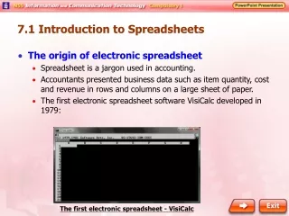
What is an electronic spreadsheet? It is the electronic equivalent of an accounting worksheet, comprised of rows and columns to allow you to do many tasks in the organization of numbers in a clear, easy to understand format
What is an electronic spreadsheet? • It is a tool to help you calculate budgets, do economic analysis, statistics, planning, engineering calculations, … • Replaces pen, paper and pocket calculator • Can show diagrams and graphs • Can input data from other programs • Can output data to other programs
Some Advantages of Spreadsheets • Spreadsheets are capable of exploring “what-if”scenarios (e.g. budgets, submitting bids) • Once it is set up properly, the user can save time by never having to set up the spreadsheet again • Blank spreadsheets are called templates. • Monthly salaries,grade sheets
Spreadsheet terminology • Row- horizontal axis (designated by numbers) • Column- vertical axis (designated by letters) • Cell - intersection of row and column (designated by an address comprised of the column letter and row number e.g. A1) • Block//Range- a rectangular group of one or more cells (identified by block coordinates (e.g. A1:G4)
Spreadsheet terminology (con’t.) • Label- alphanumeric • Value - a number or formula result • Formula- creates relationships among other cells • Template - a notebook that has labels, formulas, and all of the formatting but no actual data (e.g. actual figures and numbers)
How big is a spreadsheet? • Normally you see 9 columns and 18 rows • = 162 cells • One sheet has 256 columns and 65536 rows • = 1677216 cells • That is more than 103000 screens • Would take 34000 A4 pages to print • Take 194 days to fill at one cell pr second
Exploring the Excel Screen Title bar Menu toolbar Standard toolbar Formatting toolbar Screen Tip Active worksheet in workbook window Task Pane: organizes related commands
Activating Toolbars Click on View and Toolbars Toolbars sub-menu appears Click on desired toolbar Check indicates active item; click to deactivate
Moving Around the Worksheet Working in an active cell(intersection of a row and column) Insertion point: where text will be entered I-beam: to place insertion point Cell pointer
Moving Around the Worksheet • Move cell pointer • arrow keys • scroll bars • Change pages • click on tabs • tab scroll buttons
Moving Around the Worksheet • Consider cell B4 active • Note • thick cross mouse pointer • row, column buttons highlighted • After scrolling to right, note … • row button still highlighted • name box still shows B4 as active cell
Moving Around the Worksheet • To select a column • Click on the column heading button • Whole column is highlighted
Entering Labels • Click desired cell to make it active • Label is displayed both in cell and in formula bar as you type • Label displays out of its column • as long as other columns are empty
Worksheet with Labels • Note • Documentationsection • Label cut off, next celloccupied • Labels aligned left
Editing a Cell's Information • Click on desired cell • Cell pointer moves there • Contents displayed in formula bar • Click mouse pointer (I-beam) to location within text • type, delete, copy, paste as needed I
Entering Values • When entering numbers • do not use commas • numbers are right justified by default • To proceed to next cell right use [Tab] or right arrow key • To proceed down, use [Enter] key
Entering Formulas • Formulas are mathematical equations • perform calculations • always start with an equal sign (=) • Formula shows informula bar • Note color referencesin formula . . .
Entering Formulas • After formula entered and cell pointer moved • Formula does not show in formula bar • Result of calculations shows in cell where formula entered
Operators • ^- exponents • +- addition • * - multiplication • / - division • - - subtraction • =- function
Order Calculations are Performed • First exponents • Then any multiplication and division in the order they occur • Then any addition and subtraction in the order they occur
Parentheses • Operations within parentheses are performed before those outside. • Within the parentheses the basic rules are followed. • Multiple sets of parentheses, the innermost are executed first followed by the next set.
Built-in functions • Functions are pre-written formulas • Functions must start with an equal sign • Functions takes value(s), perform an operation, and returns a value(s) • Values you use with a function are arguments • =AVERAGE(D3:D7) • AVERAGE is the function • D3:D7 is the argument
Using Functions • Advantages of predefined functions • save time • more accurate • Using AutoSum • Click cell atbottom of column • Click AutoSumbutton • Excel assumesit should totalthe column • SUM functioninserted
Using Functions • AutoSum can also be used to right of a row of numbers
Using Functions • Note end results of using AutoSum • Note: • Click AutoSum button once to display formula,again to apply • SUM formuladisplays in Formula bar
Using the Function Insert Feature • Click on Insert, and Function • Insert Function dialog box appears Select function category Choose specific function desired
Arguments of function must be specified Note calculated result of inserted function Animated border shows selected range Formula appears in cell Using the Function Insert Feature
Note calculated result of inserted function Using the Function Insert Feature
Click on Next button to proceed Creating a Chart • Select series of numbers from worksheet • Click Chart Wizardbutton • Dialog box opens • Choose charttype, sub-type • Note previewbutton
Creating a Chart • Step 2 • Review and change series range asneeded • Click CategoryLabelsbutton to specifysource of labelsfor chart
Click on Next button to proceed Creating a Chart • Labels now show inlegend • Range for labelsnow displayed
Click on Next button to proceed Creating a Chart • Step 3 • Enter titles (whichwill show on preview) • Specify legend detailson legend tab • Specify Data Label details as shown
Creating a Chart • Step 4 • Specify where chart will appear • Click Finish
Creating a Chart • Chart is displayed as object in worksheet Note Chart toolbar displayed while chart is selected
Statistical analysis in Excel • you can do a range of statistics in Excel using the ‘Analysis ToolPak’ • you can calculate a correlation matrix and undertaking regression analysis • results of this analysis goes on additional sheets in the Excel workbook. remember to save this workbook often (as a .xls format file) • note, Excel is powerful but it is not a statistics package. Alternatives are SPSS and Minitab which are full function statistics packages and will do lots more. they will read Excel spreadsheets and dbf format data files
Opening the ToolPak, Excel’s data analysis add-in go to ‘Tools’ -> ‘Add-Ins’ choose ‘Analysis ToolPak’ and click ‘OK’
Correlation analysis • are A and B related? • correlation coefficient provides a single numerical value describing a linear relationship, telling us the direction and strength
you can get Excel to add • the ‘best fit’ line (Trendline) • through the scatter of points • to do this select the data points • on the chart, right-click and • choose ‘Add Trendline’ • In the ‘Add Trendline’ box • choose ‘Type’ - ‘Linear’ and • click ‘OK’
What do you think r will be?? • now we want to calculate the actual Pearson’s correlation • coefficient (the r value) for this relationship • it is very easy to calculate with Excel
go back to the ‘Tools’ • menu and select ‘Data Analysis’ In the ‘Data Analysis’ window choose ‘Correlation’
Correlation analysis • this window allows you to • define the variables you want • to correlate • you will correlate all your • census variables to get a full • correlation matrix • the ‘Input Range:’ box defines the columns in the spreadsheet • you want to run the correlation on. click in this box and then • with the mouse select all the columns of census data • check the ‘Labels in First Row’ box as well. make sure the • ‘New Worksheet Ply:’ option is checked and call it ‘correlation’ • and then click on ‘OK’
Steps in Developing a Spreadsheet 1. Determining the purpose- what inputs, what outputs, what printed reports 2. Planning- plan it on paper first 3. Building and testing- make sure it manipulates the data correctly 4. Documenting- should include something within the worksheet itself (directions, name and date)