Optimization and least squares
330 likes | 352 Vues
Learn about image transformations and least squares techniques in computer science with Professor Noah Snavely. Topics include convex hulls, object recognition, linear regression, residual errors, least squares fitting, and gradient descent. Explore practical methods for optimizing transformations and solving systems of equations. Discover how to apply these optimization principles to enhance image processing algorithms and object recognition systems.

Optimization and least squares
E N D
Presentation Transcript
Optimization and least squares Prof. Noah Snavely CS1114 http://cs1114.cs.cornell.edu
Administrivia • A5 Part 1 due tomorrow by 5pm (please sign up for a demo slot) • Part 2 will be due in two weeks (4/17) • Prelim 2 on Tuesday 4/7 (in class) • Covers everything since Prelim 1, including: • Polygons, convex hull, interpolation, image transformation, feature-based object recognition, solving for affine transformations • Review session on Monday, 7pm, Upson 315
Image transformations • What happens when the image moves outside the image boundary? • Previously, we tried to fix this by changing the transformation:
Image transformations • Another approach: • We can compute where the image moves to • in particular the minimum row and the minimum column • as well as the width and height of the output image (e.g., max_col – min_col + 1) • Then we can “shift” the image so it fits inside the output image • This could be done with another transformation, but could also just add/subtract min_col and min_row
Shifting the image • need to shift (row, col) by adding (min_row, min_col), before applying T-1 matrix entry (1,1) (30, -10) h (-15, -50) w
Convex hulls • If I have 100 points, and 10 are on the convex hull • If I add 1 more point • the max # of points on the convex hull is 11 • the min # of points on the convex hull is 3 new point
Object recognition • Detect features in two images • Match features between the two images • Select three matches at random • Solve for the affine transformation T • Count the number of inlier matches to T • If T is has the highest number of inliers so far, save it • Repeat 3-6 for N rounds, return the best T
When this won’t work • If the percentage of inlier matches is small, then this may not work • In theory, < 50% inliers could break it • But all the outliers would have to fit a single transform • Often works with fewer inliers
A slightly trickier problem • What if we want to fit T to more than three points? • For instance, all of the inliers we find? • Say we found 100 inliers • Now we have 200 equations, but still only 6 unknowns • Overdetermined system of equations • This brings us back to linear regression
Linear regression, > 2 points • The line won’t necessarily pass through any data point (yi, xi) y = mx + b
Some new definitions • No line is perfect – we can only find the best line out of all the imperfect ones • We’ll define a function Cost(m,b) that measures how far a line is from the data, then find the best line • I.e., the (m,b) that minimizes Cost(m,b) • Such a function Cost(m,b) is called an objective function • You learned about these in section yesterday
Line goodness • What makes a line good versus bad? • This is actually a very subtle question
Residual errors • The difference between what the model predicts and what we observe is called a residual error (i.e., a left-over) • Consider the data point (x,y) • The model m,b predicts (x,mx+b) • The residual is y – (mx + b) • For 1D regressions, residuals can be easily visualized • Vertical distance to the line
Least squares fitting This is a reasonable cost function, but we usually use something slightly different
Least squares fitting We prefer to make this a squared distance Called “least squares”
Why least squares? • There are lots of reasonable objective functions • Why do we want to use least squares? • This is a very deep question • We will soon point out two things that are special about least squares • The full story probably needs to wait for graduate-level courses, or at least next semester
Gradient descent • You learned about this in section • Basic strategy: • Start with some guess for the minimum • Find the direction of steepest descent (gradient) • Take a step in that direction (making sure that you get lower, if not, adjust the step size) • Repeat until taking a step doesn’t get you much lower
Gradient descent, 1D quadratic • There is some black magic in setting the step size
Some error functions are easy • A (positive) quadratic is a convex function • The set of points above the curve forms a (infinite) convex set • The previous slide shows this in 1D • But it’s true in any dimension • A sum of convex functions is convex • Thus, the sum of squared error is convex • Convex functions are “nice” • They have a single global minimum • Rolling downhill from anywhere gets you there
Consequences • Our gradient descent method will always converge to the right answer • By slowly rolling downhill • It might take a long time, hard to predict exactly how long (see CS3220 and beyond)
What else about LS? • Least squares has an even more amazing property than convexity • Consider the linear regression problem • There is a magic formula for the optimal choice of (m,b) • You don’t need to roll downhill, you can “simply” compute the right answer
Closed-form solution! • This is a huge part of why everyone uses least squares • Other functions are convex, but have no closed-form solution, e.g.
Closed form LS formula • The derivation requires linear algebra • Most books use calculus also, but it’s not required (see the “Links” section on the course web page) • There’s a closed form for any linear least-squares problem
Linear least squares • Any formula where the residual is linear in the variables • Examples: • simple linear regression: [y – (mx + b)]2 • finding an affine transformation [x’ – (ax + by + c)]2 + [y’ – (dx + ey + f)]2 • Non-example: [x’ – abc x]2 (variables: a, b, c)
Linear least squares • Surprisingly, fitting the coefficients of a quadratic is still linear least squares • The residual is still linear in the coefficients β1, β2, β3 Wikipedia, “Least squares fitting”
Optimization • Least squares is an example of an optimization problem • Optimization: define a cost function and a set of possible solutions, find the one with the minimum cost • Optimization is a huge field
Optimization strategies • From worse to pretty good: • Guess an answer until you get it right • Guess an answer, improve it until you get it right • Magically compute the right answer • For most problems 2 is the best we can do • Some problems are easy enough that we can do 3 • We’ve seen several examples of this
Sorting as optimization • Set of allowed answers: permutations of the input sequence • Cost(permutation) = number of out-of-order pairs • Algorithm 1: Snailsort • Algorithm 2: Bubble sort • Algorithm 3: ???
p4 minimize p1 p3 f (R,T,P) p2 p5 p7 p6 Another example: “structure from motion” Camera 1 Camera 3 R3,t3 R1,t1 Camera 2 R2,t2
Optimization is everywhere • How can you give someone the smallest number of coins back as change? • How do you schedule your classes so that there are the fewest conflicts? • How do you manage your time to maximize the grade / work tradeoff?
