
Exploring Shading Techniques in Computer Graphics
E N D
Presentation Transcript
Shading Chapter 6
Introduction: • We have learned to build three-dimensional models and to display them. • However, if you render one of our models, you might be disappointed to see images that look flat. • This appearance is a consequence of our unnatural assumption that each surface is lit such that it appears to the viewer in a single color. • We have left out the interaction between light and the surfaces in our models • So, we will begin by developing models of light sources and the most common light-material interactions. Chapter 6 -- Shading
We then will investigate how we can apply shading to a polygonal model. • We then develop a recursive approximation to a sphere to test our shading algorithms. • We then discuss how light and material properties are specified in OpenGL • and can be added to our sphere approximating program. • We conclude the chapter with a short discussion of the two most important methods for handling global lighting effects: • Ray Tracing and Radiosity Chapter 6 -- Shading
1. Light and Matter • From a physical perspective, a surface can either • emit light by self-emission (as a light bulb does) • or reflect light from other surfaces that illuminate it. Chapter 6 -- Shading
The equation for solving this shading is called the rendering equation. • This cannot be solved in general, so we use approximations. • Radiosity and ray-tracing are approximations to this. • Unfortunately these approximations cannot yet be used to render scenes at the rate we can pass polygons through the modeling-projection pipeline. • Therefore, we will focus on a simpler rendering model • This model is based upon the Phong reflection model Chapter 6 -- Shading
To get an overview of the process, we can start following rays of light from a point-light-source Chapter 6 -- Shading
In terms of Computer graphics, we replace the viewer with the projection plane • Note that most rays leaving a source do not contribute to the image and are thus of no interest to us. Chapter 6 -- Shading
The interaction between light and materials can be classified into three groups • (a) specular • (b) diffuse • (c) translucent Chapter 6 -- Shading
Specular Surfaces • appear shiny because most of the light that is reflected is reflected in a narrow range of angles close to the angle of reflection. • Angle of Incidence is equal to the angle of reflection. • Diffuse Surfaces • reflected light is scattered in all directions. • Translucent Surfaces • allow some light to penetrate the surface and to emerge from another location on the object. • Refraction Chapter 6 -- Shading
2. Light Sources • Light can leave a surface through • self-emission and reflection. • When we discuss OpenGL lighting in section 7 we shall see that we can easily simulate a self-emission term. Chapter 6 -- Shading
If we consider a source such as: • each point on the surface can emit light that is characterized by • the direction of emission (q,f) (u,t) • the intensity of energy emitted at each wavelength l • Thus, a general light source can be characterized by an illumination function • I(x, y, z, q, f, l) Chapter 6 -- Shading
From the perspective of the surface that is being illuminated, we can obtain the total contribution of the source by integrating over the surface of the source. • This can be difficult, so we will consider four basic types of sources: • ambient lighting, point sources, spotlights, and distant lights • These four are sufficient for rendering most simple scenes. Chapter 6 -- Shading
2.1 Color Sources • Not only do light sources emit different amounts of light at different frequencies, but also their directional properties can very with frequency. • Consequently, a physically correct model can be complex. • However, since we our visual system is based upon three colors, • for most applications, we can use each of the three colors to obtain what the human observer sees. Chapter 6 -- Shading
2.2 Ambient Light • In some rooms, such as certain classrooms or kitchens, the lights have been designed and positioned to provide uniform illumination throughout the room. • Often this is achieved with light sources that have diffusers whose purpose is to scatter light in all directions. • Florescent lights have covers designed to do this. Chapter 6 -- Shading
Making such a model and rendering the scene with it would be a daunting task for a graphics system. • Alternatively, we can look at the desired effect: • to achieve a uniform light level in the room • This uniform lighting is called Ambient Light. Chapter 6 -- Shading
2.3 Point Sources • An ideal point source emits light equally in all directions. • We can characterize a point light source by a three-component color matrix. • The intensity of illumination received from a point source is proportional to the inverse square of the distance from the source to the surface. Chapter 6 -- Shading
Scenes rendered with only point sources tend to have high contrast • (objects appear either bright or dark) • In the real world, it is the large size of most light sources that contributes to softer scenes. • Umbra • Penumbra Chapter 6 -- Shading
2.4 Spotlights • spotlights are characterized by a narrow range of angles through which light is emitted. • We can construct a spotlight from a point source by limiting the angles. • For example, we can use a cone Chapter 6 -- Shading
More realistic spotlights are characterized by the distribution of light in the cone. • Usually most of the light is concentrated at the center of the cone. • The intensity is a function of the angle f • As we will see throughout this chapter, cosines are convenient functions for lighting calculations. Chapter 6 -- Shading
2.5 Distant Light Sources • Most shading calculations require the direction from the point on the surface to the light source • As we move across a surface, calculating the intensity at each point, we should recompute this vector repeatedly. • This is very expensive and is a significant part of the shading calculation. • However, if the light source is far from the surface, the vector does not change much Chapter 6 -- Shading
In this case, we are effectively replacing a point light source with a source that illuminates objects with parallel rays of light. • Graphics systems can carry out rendering calculations more efficiently for distant light sources than for near ones. • OpenGL allows both Chapter 6 -- Shading
3. The Phong Reflection Model • Although we could approach light-material interactions through physical models, • we have chosen to use a model that leads to efficient computations and to be a close enough approximation to physical reality to produce good renderings under a variety of lighting conditions and material properties. Chapter 6 -- Shading
The model uses the four vectors shown here to calculate a color for a point p on a surface. • n is the normal vector at p • We discuss its computation in section 6.4 • v is the vector from p to the viewer or COP • l is the vector from p to a light source • r is in the direction that a perfectly reflected ray from l would take. • This is determined by n and l (calculated in 6.4) Chapter 6 -- Shading
The Phong model supports three types of light-material interactions • Ambient, Diffuse, and Specular. • For the total Intensity we write: • I = Ia + Id + Is = LaRa + LdRd + LsRs • where R is the reflection term • with the understanding that the computation will be done for each of the primaries and each source. Chapter 6 -- Shading
3.1 Ambient Reflection • The intensity of ambient light La is the same at every point on the surface. • Some light is absorbed and some is reflected. • The amount reflected is given by the ambient reflection coefficient, Ra=ka (0 £ ka£ 1) • Thus Ia = ka La • A surface has of course, three ambient coefficients • kar, kag, and kab • and they can be different • Hence, a sphere appears yellow under white ambient light if its blue ambient coefficient is small and its red and green coefficients are large. Chapter 6 -- Shading
3.2 Diffuse Reflection • A perfectly diffuse reflector scatters the light that it reflects equally in all directions. • Perfectly diffuse surfaces are so rough that there is no preferred angle of reflection Chapter 6 -- Shading
3.3 Specular Reflection • If we employ only ambient and diffuse reflections, our images will be shaded and will appear three-dimensional, but all the surfaces will look dull, somewhat like chalk. • What is missing is the highlights Chapter 6 -- Shading
A specular surface is smooth. • A mirror is a perfectly specular surface. • Modeling specular surfaces realistically can be complex • This is because the pattern is not symmetric, it depends upon the wavelength and it changes with the reflection angle. • The Phong model adds a term for specular reflection. • The amount of light that the viewer sees depends upon the angle f between r and the reflector v Chapter 6 -- Shading
The Phong Model uses the equation • Is = ksLscosaf • ksis the fraction of the incoming specular light that is reflected. • a is the shininess coefficient. • As a is increased, the reflected light is concentrated in a narrower region, centered on the perfect reflector. Chapter 6 -- Shading
4. Computation of Vectors • The illumination and reflection models that we have derived are sufficiently general that they can be applied to either curved or flat surfaces, to parallel or perspective views, and to distant or near surfaces. • Most require vectors and dot products. • In this section we see what additional techniques can be applied when our objets are composed of flat polygons. Chapter 6 -- Shading
4.1 Normal Vectors • Plane • Typically the definition is given as • ax+ by+ cz + d = 0 • It could also be given as • n . (p-p0) = 0 • If we were given 3 noncollinear points, we could find the normal by • n = (p2-p0) x (p1-p0) • we must be careful about the order of the vectors. Reversing the order changes the surface from outward pointing to inward pointing. Chapter 6 -- Shading
Curved Surfaces • We could go through the math of how a sphere is defined. • We could go through parametric equations of a sphere • But we are only interested in the direction of the normal, so if the sphere is centered at the origin, we can say the normal is p Chapter 6 -- Shading
In OpenGL we can associate a normal with a vertex through functions such as • glNormal3f(nx, ny, nz); • glNormal3fv(pointer_to_normal); • Normals are modal variables. • If we define a normal before a sequence of vertices • this normal is associated with all the vertices • and is used for the lighting calculations at all the vertices • The problem remains, however, that we have to determine these normals ourselves. Chapter 6 -- Shading
4.2 Angle of Reflection • Once we have calculated the normal at a point, we can use this normal and the direction of light to compute the direction of a perfect reflection • angle of incidence is equal to the angle of reflection Chapter 6 -- Shading
4.3 Use of the Halfway Vector • If we use the Phong model with specular reflections in our rendering, the dot product r.v should be recalculated at every point on the surface • We can obtain an interesting approximation by using the unit vector halfway between the viewer vector and the light-source vector: Chapter 6 -- Shading
If we replace r.v with n.h, we avoid calculation of r • However, the halfway angle is smaller than the angle used for specular computation, so if we use the same exponent e in (n.h)e the specular highlights will be smaller, • so we use a different value of e to fix this. • Exercise 6.8 helps you see how much work this saves. Chapter 6 -- Shading
4.4 Transmitted Light • Consider a surface that transmits all the light that strikes it • If the speed of light differs in the two materials, the light is bent at the surface • Let hl and ht be the indices of refraction • Snell’s law states that Chapter 6 -- Shading
Therefore, we can calculate the direction of the transmitted light. • A more general expression for what happens at a transmitting surface corresponds to this figure • some light is transmitted, • some is reflected, • and the rest is absorbed. Chapter 6 -- Shading
5. Polygonal Shading • Assuming that we can compute normal vectors, given a set of light sources and a viewer, both the lighting and illumination models that we have developed can be applied at every point on a surface. • Consider the polygon mesh shown here. We will consider three ways to shade the polygons: flat, interpolative or Gourand, and Phong shading Chapter 6 -- Shading
5.1 Flat Shading • The three vectors - l, n, and v - can vary • but for a flat polygon, n is constant • if we assume the viewer does not change, v is constant • if the light source is distance, l is constant • If all three are constant, the shading calculations only need to be carried out once for each polygon. • In OpenGL we specify flat shading through • glShadeModel(GL_FLAT); • This can be disappointing in its results Chapter 6 -- Shading
5.2 Interpolative and Gourand Shading • If we use: • glShadeModel(GL_SMOOTH); • Then OpenGL interpolates colors for other primitives like lines • The normals are computed at each vertex. Colors and intensities of interior points are interpolated between vertices. • Problem: normals are discontinuous at the vertex • Solution: average them • Color plates 3-5 show flat shading up to interpolative. Chapter 6 -- Shading
5.3 Phong Shading • Even the smoothness introduced by Gourand shading may not prevent bands. • Phong proposed that instead of interpolating the intensities, interpolate the normals • and then do calculation of intensities using the interpolated normal (typically at scan conversion) • This is much smoother, but at a greater computational cost. Chapter 6 -- Shading
6. Approximation of a Sphere by Recursive Subdivision • We have used the sphere as an example curved surface to illustrate shading calculations. • However, the sphere is not an object that is supported within OpenGL • Both the GL utility library (GLU) and the GL Utility Toolkit (GLUT) contain spheres • GLU via quadric surfaces • A topic discussed in Chapter 10 • GLUT via polygonal approximation Chapter 6 -- Shading
This section develops a polygonal approximation to a sphere. • This figure shows an approximation to a sphere drawn with this code Chapter 6 -- Shading
7. Light Sources in OpenGL • OpenGL supports the four types of light sources that we just described, and allows at least 8 light sources per program. • Each light source must be individually specified and enabled • glLightfv(source, parameter, pointer_to_array) • glLightf(source, parameter, value); Chapter 6 -- Shading
There are four vector parameters that we can set • The position (or direction) of the light, the amount of ambient, diffuse, and specular light associated with a source • For example: • glEnable(GL_LIGHTING); • glEnable(GL_LIGHT0); • glLightfv(GL_LIGHT0, GL_POSITION, light0_pos); • glLightfv(GL_LIGHT0, GL_AMBIENT, ambinet0); • glLightfv(GL_LIGHT0, GL_DIFFUSE, diffuse0); • glLightfv(GL_LIGHT0, GL_SPECULAR, specular0); • Note that we must enable both lighting and the particular source. Chapter 6 -- Shading
We can also set a global ambient term that is independent of any light • glLightModel(GL_LIGHT_MODEL_AMIENT, global_ambient_data); • We can convert a source to a spotlight by choosing: • The spotlight direction (GL_SPOT_DIRECTION) • The exponent (GL_SPOT_EXPONENT) • And the angle (GL_SPOT_CUTOFF) • If we have objects that we need to have the light interact properly with both sides we may need to set • glLightModel(GL_LIGHT_MODEL_TWO_SIDED, GL_TRUE); Chapter 6 -- Shading
8. Specification of Materials in OpenGL • Material properties in OpenGL match up directly with the supported light sources and with the Phong reflection model. • We can also specify different material properties for the front and the back faces of a surface • All our reflection parameters are specified through the functions: • glMaterialfv(face, type, pointer_to_array); • glMaterialf(face, value); Chapter 6 -- Shading
For Example: • glMaterialfv(GL_FRONT_AND_BACK, GL_AMBIENT, ambient); • Note: • If both the specular and diffuse coefficients are the same (as is of the the case), we can specify both by using GL_DIFFUSE_AND_SPECULAR • To specify different front- and back-face properties, • we use GL_FRONT and GL_BACK • The shininess of a surface (the exponent in the specular-reflection term) is specified as follows: • glMatrialg(GL_FRONT, GL_SHININESS, 100.0); Chapter 6 -- Shading
OpenGL also allows us to define surfaces that have an emissive component • This characterizes self-luminous sources. • This is useful if you want a light source to appear in your image. • It is unaffected by any light source • And it does not affect any other surface. • For example this defines a small amount of blue-green emission: • Glfloat emission[ ] = {0.0, 0.3, 0.3, 1.0}; • glMaterialfv(GL_FRONT_AND_BACK, GL_EMISSION, emission); Chapter 6 -- Shading