Estimating Electric Fields from Sequences of Vector Magnetograms
180 likes | 383 Vues
Estimating Electric Fields from Sequences of Vector Magnetograms. George H. Fisher, Brian T. Welsch, William P. Abbett, and David J. Bercik University of California, Berkeley. Why should we care about determining electric fields?.

Estimating Electric Fields from Sequences of Vector Magnetograms
E N D
Presentation Transcript
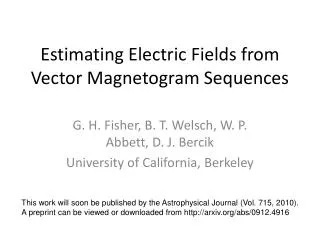
Estimating Electric Fields from Sequences of Vector Magnetograms George H. Fisher, Brian T. Welsch, William P. Abbett, and David J. Bercik University of California, Berkeley
Why should we care about determining electric fields? Electric fields on the solar surface determine the flux of magnetic energy and relative magnetic helicity into flare and CME-producing parts of the solar atmosphere: Here,EM/t is the change in magnetic energy in the solar atmosphere, and dH/dt is the change of magnetic helicity of the solar atmosphere. The flow field v is important because to a good approximation, E =-v/c x B in the layers where the magnetic field is measured. Here E is the electric field, B is the magnetic field, and Apis the vector potential of the potential magnetic field that matches its measured normal component.
Approaches to Computing Electric Fields from Magnetograms: • Assume E=-v/cxB and find v from local correlation tracking techniques applied to changes in line-of-sight magnetograms (e.g. FLCT method of Fisher & Welsch, or many others methods) • Use vector magnetograms and normal component of induction equation to determine 3 components of v (e.g. ILCT method of Welsch et al (2004), MEF method of Longcope (2004), and DAVE4VM (Schuck 2008) • Use vector magnetograms to solve all 3 components of the induction equation (this talk)
Can we determine the 3D electric field from vector magnetograms? Kusano et al. (2002, ApJ 577, 501) stated that only the equation for the normal component of B (Bz) can be constrained by sequences of vector magnetograms, because measurements in a single layer contain no information about vertical derivatives. Nearly all current work on deriving flow fields or electric fields make this same assumption. But is this statement true?
The magnetic induction equation Use the poloidal-toroidal decomposition of the magnetic field and its partial time derivative: One can then derive these Poisson equations relating the time derivative of the observed magnetic field B to corresponding time derivatives of the potential functions: Since the time derivative of the magnetic field is equal to -cxE, we can immediately relate the curl of E and E itself to the potential functions determined from the 3 Poisson equations:
Relating xE and E to the 3 potential functions: The expression for E in equation (7) is obtained simply by uncurling equation (6). Note the appearance of the 3-d gradient of an unspecified scalar potential ψ. The induction equation can be written in component form to illustrate precisely where the depth derivative terms Ey/z and Ex/z occur:
Does it work? First test: From Bx/t, By/t,Bz/t computed from Bill’s RADMHD simulation of the Quiet Sun, solve the 3 Poisson equations with boundary conditions as described, and then go back and calculate B/t from equation (12) and see how well they agree. Solution uses Newton-Krylov technique: By/t RADMHD Bz/t RADMHD Bx/t RADMHD Bz/t vs Bz/t By/t derived Bz/t derived Bx/t derived Bx/t vs Bx/t
Comparison to velocity shootout case: Bz/t ANMHD Bx/t ANMHD By/t ANMHD Bx/t derived By/t derived Bz/t derived
Velocity shoot out case (cont’d) Ex Ey Ez Ey derived Ez derived Ex derived
Summary: excellent recovery of xE, only approximate recovery of E. Why is this? The problem is that E, in contrast to xE, is mathematically under-constrained. The gradient of the unknown scalar potential in equation (13) does not contribute to xE, but it does contribute to E. In the two specific cases just shown, the actual electric field originates largely from the ideal MHD electric field –v/c x B. In this case, E∙B is zero, but the recovered electric field contains significant components of E parallel to B. The problem is that the physics necessary to uniquely derive the input electric field is missing from the PTD formalism. To get a more accurate recovery of E, we need some way to add some knowledge of additional physics into a specification of ψ. We will now show how simple physical considerations can be used to derive constraint equations for ψ.
One Approach to finding ψ: A Variational Technique The electric field, or the velocity field, is strongly affected by forces acting on the solar atmosphere, as well as by the strong sources and sinks of energy near the photosphere. Here, with only vector magnetograms, we have none of this detailed information available to help us resolve the degeneracy in E from ψ. One possible approach is to vary ψ such that an approximate Lagrangian for the solar plasma is minimized. The Lagrangian for the electromagnetic field itself is E2-B2, for example. The contribution of the kinetic energy to the Lagrangian is ½ ρv2, which under the assumption that E = -v/c x B, means minimizing E2/B2. Since B is already determined from the data, minimizing the Lagrangian essentially means varying ψ such that E2 or E2/B2 is minimized. Here, we will allow for a more general case by minimizing W2E2 integrated over the magnetogram, where W2 is an arbitrary weighting function. Note that minimizing E2/B2, i.e. setting W2=1/B2, should be equivalent to Longcope’s Mininum Energy Fit (2004, ApJ 612, 1181) solution for the magnetic field, except that in his case only the normal component of the induction equation was solved.
A variational approach (cont’d) Here the x,y,z components of EI are assumed to be taken from equation (7) without the ψ contribution. To determine ψ/z contribution to the Lagrangian functional, we can use the relationship E∙B=R∙B where R is any non-ideal contribution to E. Performing the Euler-Lagrange minimization of equation (8) results in this equation:
A variational approach (cont’d) Evaluating the equation explicitly results in this elliptic 2nd order differential equation for ψ: We have pursued numerical solutions of this equation, along with the 3 Poisson equations described earlier. Comparisons with the original ANMHD electric fields were poor. This may be due to numerical problems associated with the large dynamic range of the magnetic field-dependent coefficients in this equation. A more promising approach was recently suggested by Brian Welsch. Writing Eh = EhI-hψ, and noting that EzBz=R∙B-Bh∙Eh, equation (10) can be re-written and simplified as
A variational approach (cont’d) Equation (12) implies that we can write Dividing by W2 and then taking the divergence of this equation, we derive an elliptic equation for χ that involves the magnetic field or its time derivatives:
A variational approach (cont’d) If the non-ideal part of the electric field R is known or if one desires to specify how it varies over the magnetogram field of view, equation (14) can incorporate non-ideal terms in its solution. However, we anticipate that most of the time, the non-ideal term will be much smaller than ideal contributions, and can be set to 0. Once χ has been determined, it is straightforward to derive the electric field and the Poynting flux S=(c/4π)ExB:
A variational approach (cont’d) Finally, if one can ignore the non-ideal RB term in equation (14), then the two special cases of W2B2=1(minimized kinetic energy) and W2=1 (minimized electric field energy) result in these simplified versions of equation (14) for χ: Boundary conditions for χ are not clear, but if the outer boundary of the magnetogram has small or zero magnetic field values, it is likely that the horizontal Poynting flux, and hence ∇hχ, has a small flux normal to the magnetogram boundary. Therefore we anticipate that Neumann boundary conditions are the most appropriate for applying to χ if the boundaries are in low field-strength regions. Note that once χ has been solved for, the potential field contribution can be found by subtracting the PTD solutions for EI from the electric field from equations (15-16).
A Variational Approach (cont’d) Sx Sy Sz Sz (var) Sx (var) Sy (var)
Summary of 3D electric field inversion • It is possible to derive a 3D electric field from a time sequence of vector magnetograms which obeys all components of the Maxwell Faraday equation. This formalism uses the Poloidal-Toroidal Decomposition (PTD) formalism. • The PTD solution for the electric field is not unique, and can differ from the true solution by the gradient of a potential function. The contribution from the potential function can be quite important. • An equation for a potential function, or for a combination of the PTD electric field and a potential function, can be derived from variational principles and from iterative techniques. • The development and testing of numerical techniques are currently underway.