Download
1 / 19
190 likes | 324 Vues
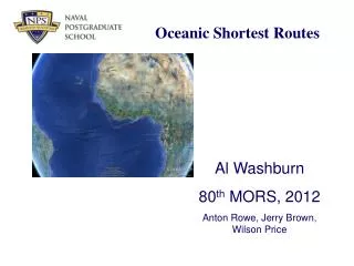
Oceanic Shortest Routes. Al Washburn 80 th MORS, 2012 Anton Rowe, Jerry Brown, Wilson Price. Underway Replenishment. A Traveling Salesman problem where the cities keep moving around on the surface of a sphere, the subject of RASP.

E N D
Oceanic Shortest Routes Al Washburn 80th MORS, 2012 Anton Rowe, Jerry Brown, Wilson Price
Underway Replenishment • A Traveling Salesman problem where the cities keep moving around on the surface of a sphere, the subject of RASP. • Here we deal with a relatively simple, embedded subproblem: • How long will it take to get from X to Y? • We assume at constant speed, so time is not involved • A simple problem, were it not for various obstacles
Consider two approximation methods • Put some kind of a finite grid on the ocean, periodically calculate all shortest routes, store them, and look them up as needed. • Move X and Y to the nearest stored points • Consider winds, currents, hurricanes, etc. when defining “distance” • Suffer from inaccuracies due to finite grid • Don’t grid the ocean, and face the fact that routing calculations cannot be completed until X and Y are known. • A different kind of approximation (symmetric shortest path) • Suffer because “distance” will have to be geometric • The subject of this talk
Obstacles • Landmasses such as America and Cyprus • 41 in our current database • Each described by a clockwise “connect the dots” exercise (a spherical polygon) • The dots are called “vertexes” • The connecting arcs are called “segments” • Great circle fragments with length < π Earth radii
An interesting and useful fact about Earth • Every contiguous land mass will fit in a hemisphere • Even EurAfrica before the Suez Canal • Thank heavens the Asia-America connection is now wet! • Therefore every obstacle has a convex hull • Half of a baseball cover will not fit in a hemisphere, and therefore does not have a convex hull, but luckily Earth does not have any such obstacles • However, many obstacles on Earth are not convex
Observation • The shortest path will either go directly from X to Y, or, if X cannot “see” Y because of some intervening obstacle, the shortest path will go from X to some vertex i that is visible from X, then from i to some vertex j (the two vertexes might be the same), etc., and then finally from j to Y that is visible from j.
Therefore … • Step 1: Compute and store the shortest distances (dij) from vertex i to vertex j, for all i and j • These are the “static” computations, and can therefore take lots of time (~1000 vertexes) • Step 2: Once X and Y are known, determine which vertexes are visible from X and from Y • If Y is visible from X, the shortest route is direct, so quit • Step 3: for all feasible pairs (i,j) sum three distances and then choose the minimum (brute force) • Steps 2 and 3 are the “dynamic” computations, which must be fast
Visibility • Static and dynamic computations both depend on first establishing visibility • A symmetric relationship between X and Y • Usually obvious to a human eyeball viewing Earth • Nontrivial analytically, and the core of the problem • We have tested two analytic methods for determining visibility: the segment intersection (SI) method and the Border method
Visibility (SI method) • If X and Y are both “wet”, then X can see Y if and only if the (minimal) great circle segment connecting X to Y intersects no segment defining the border of any obstacle • Also true if X and Y are vertexes, provided one is careful about the meaning of “intersect” • One can gamble and test for an intersection with the obstacle’s convex hull • Every pair (X,Y) requires an independent visibility calculation (1000x1000x1000 static intersection tests if there are 1000 vertexes)
The Border method • Every point X has a “Border” that amounts to partitioning a circle about X into “wedges” wherein a ray from X will first encounter a certain controlling “chain” that is a continuous part of the border of some obstacle • Given the border of X, testing visibility to Y amounts to finding the bearing of Y from X, and then testing whether the distance to Y is smaller than the distance to the controlling chain or not
An obstacle and its chains A X is at the origin, each chain goes + to -
Spherical Topology As a ray from X sweeps clockwise completely around the border of an obstacle, the angle A will increase by an amount B • In Euclidean 2-D, B will be • 0 if X is outside the obstacle • 2π if X is inside the obstacle • Related to “winding numbers” • Useful in deciding whether X is wet or dry • On the surface of a sphere, B can also be • - 2π if the antipode of X is inside the obstacle
Finding the border of X whisker cursor X Cursor moves counterclockwise through 2π, whisker follows cursor
SI versus Border SI is a medium length computation, repeated for every pair (X,Y) Border is a longer length computation, repeated for every X • The border of X determines visibility to all vertexes, as well as any other point Y Border wins by an order of magnitude • Especially if X and Y are actually sets of points at which one might start or end
Shortest path summary Use the Border method to determine vertex-to-vertex visibility Determine shortest distances among vertexes • Consider Floyd-Warshall Once X and Y are determined, use the Border method to determine point-to-point and point-to-vertex visibility • Exit if X can see Y Use brute force on visible (i,j) pairs to find the best route from X to Y
An unexpected “byproduct” of our work • A Navy ship can currently find an optimal route from X to Y only by first sending a message to a Fleet Weather Center • It would therefore be useful to have a simple, web-based procedure for finding an optimal route. • Let’s call it Oceanic Route Finder!
NPS Development Complete February 2012 Available in C2RPC April 2012