Download
1 / 16
180 likes | 385 Vues
Technology Readiness Levels of Coherent Doppler Wind Lidar for Earth Orbit. by M. J. Kavaya, F. Amzajerdian, J. Yu, G. J. Koch, U. N. Singh NASA Langley Research Center to Working Group on Space-Based Lidar Winds 28 June – 1 July, 2005 Welches, Oregon. Notional Tropospheric Winds Mission

E N D
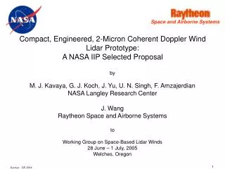
Technology Readiness Levels of Coherent Doppler Wind Lidar for Earth Orbit by M. J. Kavaya, F. Amzajerdian, J. Yu, G. J. Koch, U. N. Singh NASA Langley Research Center to Working Group on Space-Based Lidar Winds 28 June – 1 July, 2005 Welches, Oregon
Notional Tropospheric Winds Mission Vertical Profiles of Horizontal Vector Wind • 833 km sun-syn. polar orbit, on NPOESS S/C for reduced NASA cost • Step-stare conical scan, 30 deg. nadir angle, 4 az., for 2 vector wind lines (4 shown in figure) • LaRC unique high-energy 2-micron pulsed laser, 10 Hz pulse rate • 0.25 J pulse energy (1.5 J demo’d at LaRC). Derated to extend lifetime & conserve power • 120 shots per LOS wind profile (12 sec, 78 km) for better sensitivity • 20 cm optics to minimize mass, volume, alignment risk
Doppler Wind Lidar Measurement Geometry t+6.6 ms, 49 m, 6.8 mrad for return light (t+100 ms, 744 m, 103 mrad for second shot) t + 106 s 7.4 km/s 90° fore/aft angle in horiz. plane 984 km 30° FORE AFT 833 km 17 m (86%) 180 ns (27 m) FWHM (76%) 45° 34.4° 120 shots = 12 s = 78 km 492 km 348 km 1/10 s = 658 m 348 km
Notional Mission Figures of Merit 2.053 mm fundamental laser wavelength 2.053 mm transmitted laser wavelength 0.2 m physical optical diameter 0.03 m2 physical optical area 0.008 J m2 fund. l optical EAP 0.08 W m2 fund. l optical PAP 3.9 W m2 laser electrical PAP 3.9 W m2 laser orbit ave elect PAP 0.25 J fundamental laser pulse energy ~0.25 J transmitted laser pulse energy 10 Hz laser pulse rep freq, PRF 2.5 W fundamental optical power N/A fund to trans conversion efficiency ~2.5 W transmitted optical power 30 J trans opt energy/LOS wind profile 0.9 J m2 trans EAP/LOS wind profile 12 s time interval/ LOS wind profile 2% laser fundamental l WPE 125 W laser electrical power when on 100% laser pulsing duty cycle N/A laser power when not pulsing 125 W laser orbit average electrical power 60 J trans opt energy/horiz wind profile 1.9 J m2 trans EAP/horiz wind profile 118 s time interval/horiz wind profile 350 km horizontal resolution (repeat dis) 2 vector wind profiles/horiz res. 53 s time interval/horiz res. 3250 attempted vector wind profiles/day (~1700 radiosondes/day) (1 hour=3600s radiosonde time/vector profile)
Notional Tropospheric Winds Mission Vertical Profiles of Horizontal Vector Wind Courtesy: David Emmitt: • Coherent detection yields 1-2 m/s HLOS wind accuracy (RMSE) • Earth has 5668 target areas (300 x 300 km) • 14.2 orbits per day per S/C • 52% of target volumes viewed by single S/C in one day, geometry factor (blue area) • Lidar success percent ~ 50% near surface, less with increasing altitude (gray area) • Enhanced aerosol model, 2 vector wind lines, vertical resolution as shown • Repeat every 53 sec = 350 km = horizontal resolution 3250 attempted vector profiles/day (~1700 radiosondes/day) Successful profiles ~ equals radiosonde network near surface, but different global distribution Each profile covers ~ 118s, 2 x {12 s x 80 km x 25 m}
30 km 20 km 20 km < 3 m/s, N/A km < 2 m/s, 2 km Altitude ~12 ~12 < 3 m/s, 1 km 2 < 2 m/s, 0.5 km < 2 m/s, 0.5 km 2 0 0 50% 100% < 1 m/s, 0.25 km Percentage of 300 x 300 km boxes, 24 hr period 0 0 50% 100% Requirements vs. Predicted Performance Requirements – Threshold Requirements - Objective Background Aerosol Enhanced Aerosol
TRL Pros and Cons • Used by everyone in human quest to express the complex in overly simplistic terms • Many common circumstances have no guiding TRL rules for consistency: • e.g., if you take a lidar system and fly it successfully on an airplane, are you only up to TRL 4? • e.g., if you successfully space qualify a lidar system with thermal/vacuum, vibration, EMI, etc., are you up to TRL 8? • e.g., if a side-pumped laser flew successfully in space, but now you want to propose an end-pumped version, what is the TRL? (same for bandwidth, beam quality, stability, cooling technique, etc.) • e.g., if a laser flew successfully in space for a 1-year mission, but now you want to proposed a 3-year mission, what is the TRL? • e.g., if another agency/country/group of people has a successful space mission, can you take credit for TRL 9 with no guaranteed mechanism to transfer the knowledge to your mission team?
Space Coherent Doppler Lidar: TRL Levels Simultaneous Simultaneous
Space Coherent Doppler Lidar: TRL Levels Simultaneous Simultaneous
Space Coherent Doppler Lidar: TRL Levels Applies to both coherent and direct detection Doppler wind lidar
Conclusions • TRL’s don’t cover all circumstances • TRL’s are often used in an overly simplistic way • It is helpful to do a comprehensive TRL analysis • The TRL scores will vary with who is assumed to implement the mission • The gap to close for the notional mission is narrowing • Are there any suggested changes to the TRL’s shown here?
Current Wind Observations ~23.4 km • Global averages • If 2 measurements in a box, pick best one • Emphasis on wind profiles vs. height Courtesy Dr. G. David Emmitt
Supporting References • S. Chen, J. Yu, M. Petros, Y. Bai, B. C. Trieu, M. J. Kavaya, and U. N. Singh, “One-Joule Double-pulsed Ho:Tm:LuLF Master-Oscillator-Power-Amplifier (MOPA),” Advanced Solid State Photonics 20th Anniversary Topical Meeting in Vienna, Austria (Feb. 6-9, 2005) • F. Amzajerdian, B. L. Meadows, U. N. Singh, M. J. Kavaya, N. R. Baker, and R. S. Baggott, “Advancement of High Power Quasi-CW Laser Diode Arrays For Space-based Laser Instruments,” Proc. SPIE 5659, p. N/A, Fourth International Asia-Pacific Environmental Remote Sensing Symposium, Conference on Lidar Remote Sensing for Industry and Environmental Monitoring AE102, Honolulu, HI (8-12 Nov 2004) • C. P. Hale, J. W. Hobbs, and P. Gatt, “Broadly Tunable Master/Local Oscillator Lasers for Advanced Laser Radar Applications,” paper 5086-25, SPIE AeroSense 2003, Orlando, FL (21-25 April 2003) • G. J. Koch, M. Petros, B. W. Barnes, J. Y Beyon, F. Amzajerdian, J. Yu, M. J. Kavaya, and U. N. Singh, “Validar: a testbed for advanced 2-micron Doppler lidar,” Proc. SPIE 5412, Laser Radar Technology and Applications IX (12-16 April 2004)