Algorithm of Aggregate Function SUM

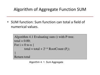
Algorithm of Aggregate Function SUM • SUM function: Sum function can total a field of numerical values. Algorithm 4.1 Evaluating sum () with P-tree. total = 0.00; For i = 0 to n { total = total + 2i * RootCount (Pi); } Return total Algorithm 4. 1. Sum Aggregate

Algorithm of Aggregate Function SUM P4,3P4,2P4,1 P4,0 0 1 1 1 0 0 0 0 1 0 1 1 1 1 10 5 6 7 11 9 3 1 0 0 0 1 1 0 1 0 1 1 1 0 1 • For example, if we want to know the total number of products which were sold out in relation S, the procedure is showed on left {3} {3} {5} {5} 51 23 * + 22 * + 21 * + 20 * =

Algorithm of Aggregate Function AVERAGE • Average function: Average function will show the average value in a field. It can be calculated from function COUNT and SUM. Average () = Sum ()/Count ().

Algorithm of Aggregate Function MAX • Max function: Max function returns the largest value in a field. Algorithm 4.2 Evaluating max () with P-tree. max = 0.00; c = 0; Pc is set all 1s For i = n to 0 { c = RootCount (Pc AND Pi); If (c >= 1) Pc = Pc AND Pi; max = max + 2i; } Return max; Algorithm 4. 2. Max Aggregate.

Algorithm of Aggregate Function MAX Steps IFPos Bits P4,3P4,2P4,1 P4,0 1. Pc = P4,3 RootCount (Pc) = 3 >=1 0 1 1 1 0 0 0 0 1 0 1 1 1 1 10 5 6 7 11 9 3 1 0 0 0 1 1 0 1 0 1 1 1 0 1 {1} {0} 2. RootCount (Pc ANDP4,2) = 0 <1 Pc = Pc AND P’4,2 3. RootCount (Pc ANDP4,1 ) = 2 >=1 Pc = Pc AND P4,1 {1} 4. RootCount (Pc ANDP4,0 ) = 1 >=1 {1} {1} {1} {1} 11 23 * + 22 * + 21 * + 20 * = {0}

Algorithm of Aggregate Function MIN • Min function: Min function returns the smallest value in a field. Algorithm 4.3. Evaluating Min () with P-tree. min = 0.00; c = 0; Pc is set all 1s For i = n to 0 { c = RootCount (Pc AND NOT (Pi)); If (c >= 1) Pc = Pc AND NOT (Pi); Else min = min + 2i; } Return min; Algorithm 4. 2. Max Aggregate.

Algorithm of Aggregate Function MIN Steps IFPos Bits P4,3P4,2P4,1 P4,0 1. Pc = P’4,3 RootCount (Pc) = 4 > =1 0 1 1 1 0 0 0 0 1 0 1 1 1 1 10 5 6 7 11 9 3 1 0 0 0 1 1 0 1 0 1 1 1 0 1 {0} 2. RootCount (Pc ANDP’4,2) = 1 >=1 Pc = Pc AND P’4,2 {0} 3. RootCount (Pc ANDP’4,1 ) = 0 <1 Pc = Pc AND P4,1 {1} 4. RootCount (Pc ANDP’4,0 ) = 0 <1 {1} {0} {0} {1} {1} 23 * + 22 * + 21 * + 20 * = 3

Algorithms of Aggregate Function MEDIAN and RANK Algorithm 4.4. Evaluating Median () with P-tree median = 0.00; pos = N/2; for rank pos = K; c = 0; Pc is set all 1s for single attribute For i = n to 0 { c = RootCount (Pc AND Pi); If (c >= pos) median = median + 2i; Pc = Pc AND Pi; Else pos = pos - c; Pc = Pc AND NOT (Pi); } Return median; • Median/Rank: Median function returns the median value in a field. • Rank (K) function returns the value that is the kth largest value in a field. Algorithm 4. 2. Median Aggregate.

Algorithm of Aggregate Function MEDIAN Steps IFPos Bits P4,3P4,2P4,1 P4,0 1. Pc = P4,3 RootCount (Pc) = 3 < 4 Pc = P’4,3 pos = 4 – 3 = 1 0 1 1 1 0 0 0 0 1 0 1 1 1 1 10 5 6 7 11 9 3 1 0 0 0 1 1 0 1 0 1 1 1 0 1 {0} 2. RootCount (Pc ANDP4,2) = 3 >=1 Pc = Pc AND P4,2 {1} 3. RootCount (Pc ANDP4,1 ) = 2 >=1 Pc = Pc AND P4,1 {1} 4. RootCount (Pc ANDP4,0 ) = 1 >=1 {1} 7 23 * + 22 * + 21 * + 20 * = {0} {1} {1} {1}

Algorithm of Aggregate Function TOP-K • Top-k function: In order to get the largest k values in a field, first, we will find rank k value Vk using function Rank (K). • Second, we will find all the tuples whose values are greater than or equal to Vk. Using ENRING technology of P-tree

Iceberg Query Operation Using P-rees • We demonstrate the computation procedure of iceberg querying with the following example: SELECT Loc, Type, Sum (# Product) FROM Relation S GROUPBY Loc, Type HAVING Sum (# Product) >= 15

PNY 1 0 1 1 0 0 0 PMN 0 1 0 0 1 0 1 PCH 0 0 0 0 0 1 0 Iceberg Query Operation Using P-trees (Step One) • Step one: We build value P-trees for the 4 values, {Loc| New York, Minneapolis, Chicago}, of attribute Loc. Figure 4. Value P-trees of Attribute Loc

LOC 0 0 0 0 1 P1,4 P1,3 P1,2 P1.1 P1.0P’1,4 P’1,3 P’1,2 P’1.1 P1.0 PNY 0 0 0 0 0 0 0 0 0 0 0 0 0 0 0 1 0 0 1 1 1 1 1 1 1 1 0 1 1 1 1 1 1 1 1 1 1 1 1 1 1 1 1 1 1 1 1 0 1 1 1 1 1 1 0 1 1 0 1 1 0 0 0 0 0 0 0 0 1 0 1 0 1 1 0 0 0 Iceberg Query Operation Using P-trees (Step One) • Figure 5 illustrates the calculation procedure of value P-tree PNY. Because the binary value of New York is 00001, we will get formula 1. PNY = P’1,4 AND P’1,3 AND P’1,2 AND P’1,1 AND P1,0 (1) Figure 5. Procedure of Calculating PNY

Iceberg Query Operation Using P-trees (Step One) • After getting all the value P-trees for each location, we calculate the total number of products sold in each place. We still use the value, New York, as our example. Sum(# product | New York) = 23 * RootCount (P4,3 AND PNY) + 22 * RootCount (P4,2 AND PNY) + 21 * RootCount (P4,1 AND PNY) + 20 * RootCount (P4,0 AND PNY) = 8 * 1 + 4 * 2 + 2 * 3 + 1 * 1 = 23 (2)

Iceberg Query Operation Using P-trees (Step One) Table 3 shows the total number of products sold out in each of the three of the locations. Because our threshold T is 15, we eliminate the city Chicago. Table 3. the Summary Table of Attribute Loc.

PNotebook PDesktop PPrinter PFAX 1 0 0 1 1 0 0 0 1 0 0 0 1 0 0 0 1 0 0 0 0 0 0 0 0 0 0 1 Iceberg Query Operation Using P-trees (Step Two) • Step two: Similarly we build value P-trees for every value of attribute Type. Attribute Type has four values {Type | Notebook, desktop, Printer, Fax}. Figure 6 shows the value P-tree of the four values of attribute Type. Figure 6. Value P-trees of Attribute Type.

Iceberg Query Operation Using P-trees (Step Two) • Similarly we get the summary table for each value of attribute Type. • According to the threshold, T equals 15, only value P-tree of notebook will be used in the future. Table 4. Summary Table of Attribute Type.

Iceberg Query Operation Using P-trees (Step Three) • Step three: We only generate candidate Loc and Type pairs for local store and Product type, which can pass the threshold T. By Performing And operation on PNY with PNotebook, we obtain value P-tree PNYAND Notebook PNY PNotebook PNY AND Notebook 1 0 1 1 0 0 0 1 0 0 1 1 0 0 1 0 0 1 0 0 0 = AND Figure 7. Procedure of Calculating PNY AND Notebook

Iceberg Query Operation Using P-trees (Step Three) • We calculate the total number of notebooks sold out in New York by formula 3. Sum(# Product | New York) = 23 * RootCount (P4,3 ANDPNY AND Notebook) + 22 * RootCount (P4,2 AND PNY AND Notebook) + 21 * RootCount (P4,1 AND PNY AND Notebook) + 20 * RootCount (P4,0 ANDPNY AND Notebook) = 8 * 1 + 4 * 1 + 2 * 2 + 1* 1 = 17 (3)

PMN PNotebook PMN AND Notebook 0 0 0 0 1 0 0 0 1 0 0 1 0 1 1 0 0 1 1 0 0 AND = Iceberg Query Operation Using P-trees (Step Three) • By performing And operations on PMN with P Notebook, we obtain value P-tree PMNAND Notebook Figure 8. Procedure of Calculating PMN AND Notebook

Iceberg Query Operation Using P-trees (Step Three) • We calculate the total number of notebook sold out in Minneapolis by formula 4. Sum (# product | Minneapolis) = 23 * RootCount (P4,3 AND PMNAND Notbook) + 22 * RootCount (P4,2 AND PMN ANDNotbook) + 21 * RootCount (P4,1 AND PMNAND Notbook) + 20 * RootCount (P4,0 AND PMNAND Notbook) = 8 * 1 + 4 * 0 + 2 * 1 + 1 * 1 = 11 (4)

Iceberg Query Operation Using P-trees (Step Three) • Finally, we obtain the summary table 5. According to the threshold T=15, we can see that only group pair “New York And Notebook” pass our threshold T. From value P-tree PNYAND Notebook, we can see that tuple 1 and 4 are in the results of our iceberg query example. PNYAND Notebook 1 0 0 1 0 0 0 Table 5. Summary Table of Our Example.

Algorithm of Aggregate Function SUM