Estuarine habitat modeling in Southeast Alaska

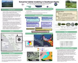
1. Estuarine habitat modeling in Southeast Alaska Jamie D. Fuller1 Sam Lischert2, Carolyn Ownby3, Wei Gao3, and Lee Benda2 Graduate Degree Program in Ecology, Colorado State University and (2) Earth Systems Institute (3) USDA UV-B Monitoring Program and ColoradoView • Research Objectives • Classification • Background To identify estuarine habitat using geomorphic variables and Landsat 8 imagery for Southeast Alaska. Identify the extent of salt marsh and mud flat area per estuarine area. Calculate total estuarine habitat for Southeast Alaska. Land-cover Classes: Salt marsh Upper Estuary –no inundation and densely vegetated Middle Estuary – occasionally inundated and vegetated Lower Estuary – frequently inundated; sparsely vegetated with salt tolerant vegetation Salt marsh-mudflat transition zone – areas not definitively salt marsh or mudflat Mud flats Mudflats – estuarine mud and silt tidal deposits; not vegetated Eelgrass – submerged/partially submerged grass-like vegetation Rocky, sandy, & glacial flow – brightly reflective deposits Transitional Forest – forest cover intermingled within the estuary or near 20 m in elevation. • Estuarine habitats in Southeast Alaska include an extensive network of intertidal mudflats and salt marshes. • Estuarine habitats are ecologically and economically important. They provide critical habitat for diverse flora and fauna, protect shorelines from erosion and flooding, support recreation and commercial fisheries, and sequester large amounts of carbon (Albert, 2010). • Delineating the variable spatial extent of estuarine habitats in Southeast Alaska will provide a better understanding of critical habitats and will lead to improved ecological mapping and classification. • Since the Little Ice Age (1700’s) rapid and widespread glacial retreat has resulted in isostatic adjustment in SE Alaska (Larsen et al, 2005). There is a strong N-S gradient in rate of uplift varying between 1 to 32 mm/yr. (Sun et al. 2010). Uplift is causing estuarine areas to enlarge over time. • Knowledge of the spatial distribution of estuaries, in combination with other watershed characteristics such as fish habitats, floodplains and network geometry, will be used to develop a watershed ecological classification scheme. • Data Processing Multispectral imagery: Landsat 8 Radiometric correction • 15 scenes cover the entire extent • were captured in 2013 between 6/10 – 8/25 • Scenes are, on average, within 2 hours of low tide Restacked bands to mimic Landsat 7 format for ENVI processing • Reclassify and multiply the DEM, Cirrus clouds, and NDVI: • 1 – region of interest (ROI) • 0 – No Data Mask probable estuary areas: Estuary Land Water mask: NDVI (values: -0.2 to 1) Cloud Mask: Landsat 8 Cirrus band Elevation Mask: ASTER Digital Elevation Model (DEM): -5 to 20 meters Ocean Add the Estuary ROI to spectral data as a band layer and apply ROI High Tide Tasseled Cap analysis Image Classification Low Tide Supervised classification: 35+ training polygons per class Method: maximum likelihood classifier Fig. 1. The various ecotones that can be found in an estuary. • Results Accuracy assessment using 55 randomly generated points per class to calculate overall accuracy and the Kappa statistic. • Results Forest transitional zone Low Estuary Upper Estuary Middle Estuary • Results Transition zone • Across the extent of this study (~1,000,000 km2) where 0.7% is estuarine habitat, the mudflat class occupies 60% or 4200 km2 and the estuary occupies 40% or 2800 km2 (Fig 3). • The differences among estuary habitats can be identified using • multispectral imagery captured proximal to low tide (Fig 3). • An accuracy assessment of 55 random points per class resulted in a good overall accuracy of 91% and Kappa statistic of 87% (Table 1). Mud flats Increasing frequency of tidal inundation and increasing salt tolerance Sea water Eelgrass 40% Fig. 3. Percentage of each estuarine land-cover class. The total mudflat areas total 4200 km2 and the estuary areas total2800 km2. Breakdown 60% Table 1. Accuracy assessment for the estuary, mudflat, and forest classifications. Fig. 4. Estuary near Gustavus showing fine resolution imagery from ESRI (left) and land-cover classification (right). • Discussion and Future Work • The estuary habitats land-cover classification for SE Alaska provides detailed information of estuary characteristics and supports continued ecological and economical research. • In other studies, isostatic rebound was shown to result in the regional uplift (Larsen et al., 2005). Next, we will pair each estuary classification, slope, and area to estimate the extent of accretion per estuary. • Estuarine classes and area data will be integrated with NetMap stream reach attributes to determine spatial relationships between estuaries and the watersheds upstream. The classification can be joined to a number of physical and biological variables (land cover, topography, watershed area, and stream geomorphology) to further inform estuarine mapping and models. Fig. 2. Southeastern Alaska spanning from Yakutat to the southern tip of Alaska. The inlay pie char shows the percentage of land-cover that is estuary. • References Albert, D., C. Shanley, and L. Baker (2010) A preliminary classification of bays and estuaries in Southeast Alaska: A hierarchical Framework and Exploratory analysis. Coastal ecological systems in Southeast Alaska, June, Nature Conservancy Report. Larsen, C. F., R. J. Motyka, J. T. Freymueller, K. A. Echelmeyer, E. R. Ivins (2005) Rapid viscoelastic uplift in southeast Alaska caused by post-Little Ice Age glacial retreat. Earth and Planetary Science Let., 237, 547-560 doi:10.1016/j.epsl.2005.06.032. Sun, W., S. Miura, T. Sato, T. Sugano, J. Freymueller, M. Kaufman, C. F. Larsen, R. Cross, and D. Inazu (2010), Gravity measurements in southeastern Alaska reveal negative gravity rate of change caused by glacial isostatic adjustment, J. Geophys. Res., 115, B12406, doi:10.1029/2009JB007194. Fig. 5. Estuary between Wrangle and Petersburg showing fine resolution imagery from ESRI (left) and land-cover classification (right).