General Rules for Dealing with Outlier Data
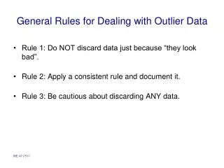
General Rules for Dealing with Outlier Data. Rule 1: Do NOT discard data just because “they look bad”. Rule 2: Apply a consistent rule and document it. Rule 3: Be cautious about discarding ANY data. Outlier Data Detection – one approach.

General Rules for Dealing with Outlier Data
E N D
Presentation Transcript
General Rules for Dealing with Outlier Data • Rule 1: Do NOT discard data just because “they look bad”. • Rule 2: Apply a consistent rule and document it. • Rule 3: Be cautious about discarding ANY data.
Outlier Data Detection – one approach • Calculate the probability that a single point would fall in the suspect range. • Multiply this probability by the number of measurements in the sample to determine the expected number of measurements in this range. • If this number is less than 0.1 then the point is an outlier. Prof. Sailor
Outlier Data Detection Keep in mind that if our sample is large enough we DO expect some points out beyond 3sigma. So, it is not just how far out a point appears, but rather, what the probability is (for the given sample size) that at least one point would be that far out. mean suspected outlier Prof. Sailor
Outlier Example 1 • Consider the case of 12 replicate measurements. X= 0.45, 0.46, 0.46, 0.47, 0.47, 0.47, 0.47, 0.48, 0.48, 0.50, 0.53, and 0.58 • Question: Are any of these data outliers? • By definition you suspect points at either end of the spectrum of values … perhaps 0.45 • …more likely 0.58 • …or possibly both 0.53 and 0.58… • …but how do we decide? Prof. Sailor
Outlier Example 1 • Consider the case of 12 replicate measurements. X= 0.45, 0.46, 0.46, 0.47, 0.47, 0.47, 0.47, 0.48, 0.48, 0.50, 0.53, and 0.58 • Mean = 0.485 • Standard Deviation = 0.036556 • N=12 • P(x>=0.58) = 0.5- 0.4953 = 0.0047 and N*P= 0.0564 (from Table 4.3 – one-sided integral) • Thus, 0.58 IS an OUTLIER! • In general you would test other points WITHOUT recalculating statistics. No other points are outliers. • We would then recalculate the statistics for presentation of results Prof. Sailor
Outlier Example 2 • Consider Example 4.11 from the text. X= 28, 31, 27, 28, 29, 24, 29, 28, 18, 27 • Mean = 26.9 • Standard Deviation = 3.604 • N=10 • P(x<=18) = 0.5- 0.4932= 0.0068 and N*P= 0.068 (from Table 4.3 – one-sided integral) • Thus, 18 IS an OUTLIER! (book gets same end result, but is casual with their roundoff and has different intermediate numbers!) Prof. Sailor
More on Outlier Analysis • Chauvenet’s criterion is also often used for outlier detection. It is similar to the approach just presented, but with a critical number P*N of 0.5 rather than 0.1 • Pierce’s criterion – more rigorous than Chauvenet’s criterion and useful for multiple suspect points. • For further options and details see various statistics texts such as: • Taylor, John R. An Introduction to Error Analysis. 2nd edition. Sausolito, California: University Science Books, 1997. Prof. Sailor
Definition of Uncertainty(Ch. 5 in Figliola and Beasley) • In most experiments, the "correct value" is not known. Rather, we are attempting to measure a quantity with less than perfect instrumentation. • The uncertainty is an estimate of the likely error. As a rule of thumb, use a 95% confidence interval. • In other words, if I state that I have measured the height of my desk to be 38 +/- 1 inch - I am suggesting that I am 95% sure that the desk is between 37 and 39 inches tall. Prof. Sailor
Uncertainty … • The producer of a particular alloy claims a modulus of elasticity of 40kPa +/- 2 kPa. What does this mean? • Answer: The general rule of thumb is that the +/- 2kPa would represent a 95% confidence interval. • That is, if you randomly select many samples of this manufacturer's alloy you should find that 95% of the samples meet the stated limit of 40 +/- 2 kPa. • This does not mean that you couldn't get a sample that has a modulus of elasticity of 43 kPa, it just means that it is very unlikely. Prof. Sailor
Uncertainty • Uncertainty vs. Error • Design Stage Uncertainty • Zero-order uncertainty: Uo = ½ resolution • Instrument uncertainty: Uc • Can be the combination (root sum squares) of individual error components (e.g., linearity & hysteresis) • Design stage uncertainty is the combination of Uo and Uc: • Propagation of Uncertainty • Euclidean Norm approach (similar to RSS) Prof. Sailor
Calculation uncertainty and the Euclidean Norm • In most experiments, several quantities are measured in order to calculate a desired quantity. For instance, if one wanted to estimate the gravitational constant by dropping a ball from a known height, the correct equation would be: g = 2L/t2 Prof. Sailor
Gravity Example and Propagating Uncertainties • Suppose we measure L = 50 m and t = 3.12 sec • How do we estimate the uncertainty in our calculation of g? • Suppose the uncertainties in the measurements are +/- 0.01 m and +/- 0.5 sec. • Based on the equation we have g= 2(50.00)/(3.1)(3.1) or g= 10.4 m/s2. Prof. Sailor
Worst Case Uncertainties • One way of looking at the uncertainty is to immediately calculate the "worst cases". • g= (2)(50.01)/(2.6)(2.6) = 14.8 m/s2 • g= (2)(49.99)/(3.6)(3.6) = 7.7 m/s2 • These would yield a confidence interval around g as: 7.7 < g <= 14.8 m/s2 • This is generally an OVERESTIMATION of uncertainty, and NOT a very good approach. Prof. Sailor
Need for a Norm • It is unlikely for all individual measurement uncertainties in a system to simultaneously be the worst possible. • So, the “worst case” approach is NOT a good one. • Some average or "norm" of the uncertainties must be used in estimating a combined uncertainty for the calculation of g. The norm that we use is called the Euclidean Norm. Prof. Sailor
Euclidian Norm Defined • In general, if the quantity Y is determined by an equation involving n independent variables Xi: • Y = f(X1,X2,X3,..., Xn), • and the uncertainty in each independent measurement variable Xi is called Ui, then the uncertainty in Y is given by: Prof. Sailor
Propagation of Uncertainty • In many instances we will simply use the design-stage uncertainty for each (of n) measurement to assess uncertainty in calculated variables: Prof. Sailor
Euclidian Norm Applied to Our Example So g= 10+/-3 m/s2. This is an example of a bad experiment. A much better in home experiment for estimating g is to use the physics behind an ideal pendulum. Prof. Sailor
Euclidian Norm Example 1 • Example: Suppose Y= AX4, where A is some known constant and X is a measured quantity (X=300 K +/- 10%). What is Y and the uncertainty in Y? • Answer: First note that we could just as easily have specified X= 300 K +/- 30 K. The estimate for Y is given by Y= A(300^4) = A* 8.1e9. • For the Euclidean norm we need to calculate one partial derivative: dY/dX. • dY/dX = 4*A*X^3. • The uncertainty in Y then is UY = sqrt ( [4*A*X^3*30 K]^2 ) • or UY = sqrt ( [4*A*(300 K)^3*30 K]^2 ) • so UY = sqrt ( 1.050e19*A^2) = A * 3.24e9 K^4 • Thus, Y= 8.1e9*A +/- 3.2e9*A , or Y= 8.1e9*A +/- 40% (units here are in K^4) Prof. Sailor