Theory of Computation 計算理論

1. Theory of Computation 計算理論

2. Instructor: 顏嗣鈞 E-mail: yen@ee.ntu.edu.tw Web: http://www.ee.ntu.edu.tw/~yen Time: 2:20-5:10 PM, Tuesday Place: BL 112 Office hours: by appointment Class web page: http://www.ee.ntu.edu.tw/~yen/courses/TOC-2006.htm

3. textbook • : Introduction to Automata Theory, Languages, andComputation John E. Hopcroft, Rajeev Motwani, Jeffrey D. Ullman, (2nd Ed. Addison-Wesley, 2001)

4. 1st Edition Introduction to Automata Theory, Languages, andComputation John E. Hopcroft, Jeffrey D. Ullman, (Addison-Wesley, 1979)

5. Grading HW : 0-20% Midterm exam.: 35-45% Final exam.: 45-55%

6. Why Study Automata Theory? Finite automata are a useful model for important kinds of hardware and software: • Software for designing and checking digital circuits. • Lexical analyzer of compilers. • Finding words and patterns in large bodies of text, e.g. in web pages. • Verification of systems with finite number of states, e.g. communication protocols.

7. Why Study Automata Theory? (2) The study of Finite Automata and Formal Languages are intimately connected. Methods for specifying formal languages are very important in many areas of CS, e.g.: • Context Free Grammars are very useful when designing software that processes data with recursive structure, like the parser in a compiler. • Regular Expressions are very useful for specifying lexical aspects of programming languages and search patterns.

8. Why Study Automata Theory? (3) Automata are essential for the study of the limits of computation. Two issues: • What can a computer do at all? (Decidability) • What can a computer do efficiently? (Intractability)

9. Applications Pattern recognition Prog. languages Supervisory control Computer-Aided Verification Comm. protocols Compiler circuits Quantum computing ... Theoretical Computer Science Automata Theory, Formal Languages, Computability, Complexity …

10. Aims of the Course • To familiarize you with key Computer Science concepts in central areas like - Automata Theory - Formal Languages - Models of Computation - Complexity Theory • To equip you with tools with wide applicability in the fields of CS and EE, e.g. for - Complier Construction - Text Processing - XML

11. Fundamental Theme • What are the capabilities and limitations of computers and computer programs? • What can we do with computers/programs? • Are there things we cannot do with computers/programs?

12. Studying the Theme • How do we prove something CAN be done by SOME program? • How do we prove something CANNOT be done by ANY program?

13. Example: The Halting Problem (1) Consider the following program. Does it terminate for all values of n  1? while (n > 1) { if even(n) { n = n / 2; } else { n = n * 3 + 1; } }

14. Example: The Halting Problem (2) Not as easy to answer as it might first seem. Say we start with n = 7, for example: 7, 22, 11, 34, 17, 52, 26, 13, 40, 20, 10, 5, 16, 8, 4, 2, 1 In fact, for all numbers that have been tried (a lot!), it does terminate . . . . . . but in general?

15. Example: The Halting Problem (3) Then the following important undecidability result should perhaps not come as a total surprise: It is impossible to write a program that decides if another, arbitrary, program terminates (halts) or not. What might be surprising is that it is possible to prove such a result. This was first done by the British mathematician Alan Turing.

16. Computability Automata Complexity Our focus

17. Topics 1.  Finite automata, Regular languages, Regular grammars: deterministic vs. nondeterministic, one-way vs. two-way finite automata, minimization, pumping lemma for regular sets, closure properties. 2.  Pushdown automata, Context-free languages, Context-free grammars: deterministic vs. nondeterministic, one-way vs. two-way PDAs, reversal bounded PDAs, linear grammars, counter machines, pumping lemma for CFLs, Chomsky normal form, Greibach normal form, closure properties. 3.

18. Topics (cont’d) 3.Linear bounded automata, Context-sensitive languages, Context-sensitive grammars. 4. Turing machines, Recursively enumerable sets, Type 0 grammars: variants of Turing machines, halting problem, undecidability, Post correspondence problem, valid and invalid computations of TMs.

19. 5. Basic recursive function theory 6. Basic complexity theory: Various resource bounded complexity classes, including NLOGSPACE, P, NP, PSPACE, EXPTIME, and many more. reducibility, completeness. 7. Advanced topics: Tree Automata, quantum automata, probabilistic automata, interactive proof systems, oracle computations, cryptography. Topics (cont’d)

20. Who should take this course? YOU

21. Languages The terms languageand wordare used in a strict technical sense in this course: A language is a set of words. A word is a sequence (or string) of symbols.  (or ) denotes the empty word, the sequence of zero symbols.

22. Symbols and Alphabets • What is a symbol, then? • Anything, but it has to come from an alphabet which is a finite set. • A common (and important) instance is = {0, 1}. •  , the empty word, is never an symbol of an alphabet.

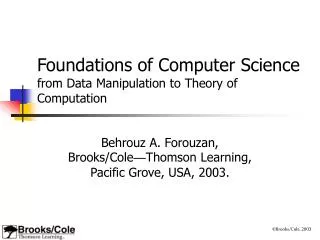
23. Computation memory CPU

24. temporary memory input memory CPU output memory Program memory

25. Example: temporary memory input memory CPU output memory Program memory compute compute

26. temporary memory input memory CPU output memory Program memory compute compute

27. temporary memory input memory CPU output memory Program memory compute compute

28. temporary memory input memory CPU Program memory output memory compute compute

29. Automaton temporary memory Automaton input memory CPU output memory Program memory

30. Different Kinds of Automata • Automata are distinguished by the temporary memory • Finite Automata: no temporary memory • Pushdown Automata: stack • Turing Machines: random access memory

31. Finite Automaton temporary memory input memory Finite Automaton output memory Example: Vending Machines (small computing power)

32. Pushdown Automaton Stack Push, Pop input memory Pushdown Automaton output memory Example: Compilers for Programming Languages (medium computing power)

33. Turing Machine Random Access Memory input memory Turing Machine output memory Examples: Any Algorithm (highest computing power)

34. Power of Automata Finite Automata Pushdown Automata Turing Machine Less power More power Solve more computational problems

35. Mathematical Preliminaries

36. Mathematical Preliminaries • Sets • Functions • Relations • Graphs • Proof Techniques

37. SETS A set is a collection of elements We write

38. Set Representations • C = { a, b, c, d, e, f, g, h, i, j, k } • C = { a, b, …, k } • S = { 2, 4, 6, … } • S = { j : j > 0, and j = 2k for some k>0 } • S = { j : j is nonnegative and even } finite set infinite set

39. U A 6 8 2 3 1 7 4 5 9 10 A = { 1, 2, 3, 4, 5 } • Universal Set: all possible elements • U = { 1 , … , 10 }

40. B A • Set Operations • A = { 1, 2, 3 } B = { 2, 3, 4, 5} • Union • A U B = { 1, 2, 3, 4, 5 } • Intersection • A B = { 2, 3 } • Difference • A - B = { 1 } • B - A = { 4, 5 } U A-B

41. Complement • Universal set = {1, …, 7} • A = { 1, 2, 3 } A = { 4, 5, 6, 7} 4 A A 6 3 1 2 5 7 A = A

42. { even integers } = { odd integers } Integers 1 odd 0 5 even 6 2 4 3 7

43. DeMorgan’s Laws A U B = A B U A B = A U B U

44. Empty, Null Set: = { } S U = S S = S - = S - S = U = Universal Set

45. U A B U A B Subset A = { 1, 2, 3} B = { 1, 2, 3, 4, 5 } Proper Subset: B A

46. A B = U Disjoint Sets A = { 1, 2, 3 } B = { 5, 6} A B

47. Set Cardinality • For finite sets A = { 2, 5, 7 } |A| = 3

48. Powersets A powerset is a set of sets S = { a, b, c } Powerset of S = the set of all the subsets of S 2S = { , {a}, {b}, {c}, {a, b}, {a, c}, {b, c}, {a, b, c} } Observation: | 2S | = 2|S| ( 8 = 23 )

49. Cartesian Product A = { 2, 4 } B = { 2, 3, 5 } A X B = { (2, 2), (2, 3), (2, 5), ( 4, 2), (4, 3), (4, 5) } |A X B| = |A| |B| Generalizes to more than two sets A X B X … X Z

50. FUNCTIONS domain range B A f(1) = a a 1 2 b c 3 f : A -> B If A = domain then f is a total function otherwise f is a partial function