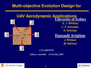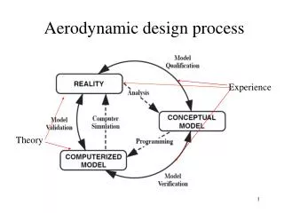
Multi-objective Evolution Design for UAV Aerodynamic Applications
Multi-objective Evolution Design for UAV Aerodynamic Applications. University of Sydney E. J. Whitney L. F. Gonzalez K . Srinivas Dassault Aviation J. Périaux M. Sefrioui. UAV-MMNT03 Sydney, Australia 14-16 July 2003. Overview. Evolution Algorithms (EAs).


Multi-objective Evolution Design for UAV Aerodynamic Applications
E N D
Presentation Transcript
Multi-objective Evolution Design for UAV Aerodynamic Applications University of Sydney E. J. Whitney L. F. Gonzalez K. Srinivas Dassault Aviation J. Périaux M. Sefrioui UAV-MMNT03 Sydney, Australia 14-16 July 2003
Overview • Evolution Algorithms (EAs). • Hierarchical Topology-Multiple Models. • Multi-Criteria Optimisation – Game Theory. • Parallel Computing and AsynchronousEvaluation. • Test Case Applications: • UAV aerofoil design for transit and loiter. • UAV aerofoil design for transit and takeoff. • UCAV whole aircraft conceptual design.
The Problem… Problems in aerodynamic optimisation: • Modern aerodynamic design uses CFD (Computational Fluid Dynamics) almost exclusively. • CFD has matured enough to use for preliminary design andoptimisation. • Most aerodynamic design problems will need to be stated in multi-objective form. • The internal workings of validated in-house solvers are essentially inaccessible from a modification point of view (they are black-boxes). • Fitness functions of interest are generally multimodal with a number of local minima. Sometimes the optimum shape/s is not obvious to the designer. The fitness function will involve some numerical noise.
… The Solution We apply an Evolution Algorithm (EA): • EAs are able to explore large search spaces. • They are robust towards noise and local minima. • They are easy to parallelise, significantly reducing computation time. • EAs successively map multiple populations of points, alowing solution diversity. • They are capable of finding a number of solutions ina Pareto set or calculating a robust Nash game.
“The Central Difficulty” Evolutionary techniques are … still … very … slow! (Often involving hundreds or thousands of separate flow computations) Therefore, we need to think about ways of speeding up the process…
Exploitation (small mutation span) Model 1 precise model Exploration (large mutation span) Model 2 intermediate model Model 3 approximate model Hierarchical Topology-Multiple Models • Interactions of the 3 layers: solutions go up and down the layers. • The best ones keep going up until they are completely refined. • No need for great precision during exploration. • Time-consuming solvers are used only for the most promising solutions. • Think of it as a kind of optimisation and population based multigrid.
Different Speeds 1 individual Asynchromous Evaluator 1 individual Parallel Computing and Asynchronous Evaluation Evolution Algorithm
No need for synchronicity no possible wait-time bottleneck. • No need for the different processors to be of similar speed. • Processors can be added or deleted dynamically during the execution. • There is no practical upper limit on the number of processors we can use. • All desktop computers in an organisation are fair game. Asynchronous Evaluation • Fitness functions are computed asynchronously. • Only one candidate solution is generated at a time, and only one individual is incorporated at a time rather than an entire population at every generation as is traditional EAs. • Solutions can be generated and returned out of order.
Multi-Criteria Problems • Aeronautical design problems normally require a simultaneous optimisation of conflicting objectives and associated number of constraints. They occur when two or more objectives that cannot be combined rationally. For example: • Drag at two different values of lift. • Drag and thickness. • Pitching moment and maximum lift. • Generation of a Pareto front allows the designer to choose after the optimisation phase; This allows selection amongst a wide range of potential solutions.
…..Multi--Criteria Optimisation A multi-criteria optimisation problem can be formulated as: Minimise: Subject to constraints: Using this concept, the objective of Pareto optimality is to find the non-dominated set of of optimum individuals (i.e. aerofoils, nozzles, wings) between a number of specified criteria.
Some More Examples Here our EA solves a two objective problem with two design variables. There are two possible Pareto optimal fronts; one obvious and concave, the other deceptive and convex.
Some More Examples (2) Again, we solve a two objective problem with two design variables however now the optimal Pareto front contains four discontinuous regions.
Nash Games • A Nash optimisation can be viewed as a competitive game between two players that each greedily optimise their own objective at the expense of the other player. • A Nash equilibrium is obtained when no player can improve his own objective at the expense of the other. Epoch Completed? Player 2 Player 1 Migrate and Exchange
Applications Now we present three UAV case studies. All have two objectives. These are: • Case One: Aerofoil design, drag minimisation for high-speed transit and loiter conditions. • Case Two: Aerofoil design, drag minimisation for high-speed transit and takeoff conditions. • Case Three: Whole aircraft conceptual design, gross weight minimisation and cruise efficiency maximisation.
Case One Problem Definition: • Dual point design procedure is described here to find the Pareto set of aerofoils for minimum total drag at two design points.The flow conditions for the two points analyzed are:
Bounding Envelope of the Aerofoil Search Space and an Example Solution • Constraints: • Thickness > 12% x/c • Pitching moment > -0.065 • Two Bezier curves representation. • Four control points on the mean line. • Five control points on the thickness distribution.
Solver • Panel method with coupled integral boundary layer (XFOIL), by M. Drela of MIT Aero-Astro. • The solver gives very good approximations of important flow features in the purely subsonic regime, including finite separation bubbles and thinly separated regions. • Free boundary layer transition is used. • Any candidate which is found to have supersonic flow regions (transonic aerofoil) is rejected immediately.
Exploitation Population size = 20 Model 1 119 Surface Panels Intermediate Population size = 20 Model 2 99 Surface Panels Model 3 79 Surface Panels Exploration Population size = 10 Hierarchical Implementation
Three discontinuous regions First Case Results
Objective Two Optimal Compromise Objective One Optimal First Case Results (2)
First Case Results (3) Objective One Optimal - Transit Condition
First Case Results (4) Compromise Solution - Transit Condition Compromise Solution - Loiter Condition
First Case Results (5) Objective Two Optimal - Loiter Condition
Case Two Problem Definition: • Again, a dual point design procedure is described here to find the Pareto set of aerofoils for minimum total drag at two design points.The flow conditions for the two points analyzed are:
Implementation • Single population used, 139 surface panels. • 6 control points on the mean line, 8 on the thickness distribution. • Run for 7,700 function evaluations. • Thickness similarly constrained (> 12%), but pitching moment only constrained for transit case.
Concave region Second Case Results
Objective Two Optimal Compromise Second Case Results (2) Objective One Optimal
Second Case Results (3) Objective One Optimal - Transit Condition
Second Case Results (4) Compromise Solution - Transit Condition Compromise Solution - Takeoff Condition
Second Case Results (5) Objective Two Optimal - Takeoff Condition
Case Three Problem Definition: • Find conceptual design parameters for a UCAV, to minimise two objectives: • Gross weight min(WG) • Cruise efficiency min(1/[MCRUISE.L/DCRUISE]) • We have six unknowns:
Cruise 40000 ft, Mach 0.9, 400 nm Release Payload 1800 Lbs Accelerate Mach 1.5, 500 nm Maneuvers at Mach 0.9 Release Payload 1500 Lbs Taxi Climb 20000 ft Descend Takeoff Landing EngineStart and warm up Mission Definition
Solver • The FLOPS (FLight OPtimisation System) solver developed by L. A. (Arnie) McCullers, NASA Langley Research Centerwas used for evaluating the aircraft configurations. • FLOPS is a workstation based code with capabilities for conceptual and preliminary design of advanced concepts. • FLOPS is multidisciplinary in nature and contains several analysis modules including: weights, aerodynamics, engine cycleanalysis, propulsion, missionperformance, takeoff and landing, noise footprint,cost analysis,and program control.
Implementation • Solved via a Nash game. • Two hierarchical trees, each with two levels and population sizes of 10. • Information exchanged (epoch) after 50 function evaluations. • Variables split: • Player One: Aspect ratio, wing thickness and wing sweep; Maximises cruise efficiency. • Player Two: Wing area, engine thrust and wing taper; Minimises gross weight. • Run for 550 function evaluations, but converged after 250.
Third Case Results (4) Upper Bound Nash Equilibrium Lower Bound
Conclusion • The multi-criteria HAPEA has shown itself to be promising for direct and inverse design optimisation problems. • No problem specific knowledge is required The method appears to be broadly applicable to black-box solvers. • A wide variety of optimisation problems including Multi-disciplinary Design Optimisation (MDO) problems can be solved. • The process finds traditional classical aerodynamic results for standard problems, as well as interesting compromise solutions. • The algorithm may attempt to circumvent convergence difficulties with the solver.
Future • Work is in progress to apply the optimisation procedure to multidisciplinary problems. We intend to couple the aerodynamic optimisation with: • Electromagnetics - Investigating the tradeoff between efficient aerodynamic design and RCS issues. • Structures - Especially in three dimensions means we can investigate interesting tradeoffs that may provide weight improvements. • Acoustics - How to maintain efficiency while lowering detectability. • And others…
E ND