Download
1 / 22
240 likes | 458 Vues
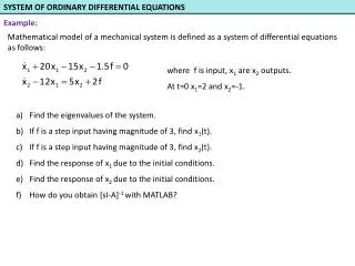
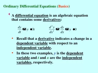
Chapter 16 Integration of Ordinary Differential Equations. Examples of Differential Equations. ODE: Newton’s equation of motion F =md 2 r /d t 2 Chemical reaction dynamics d C /d t = - C Population dynamics in ecology PDE: Maxwell equations for electricity and magnetism

E N D
Examples of Differential Equations • ODE: • Newton’s equation of motion F=md2r/dt2 • Chemical reaction dynamics dC/dt = -C • Population dynamics in ecology • PDE: • Maxwell equations for electricity and magnetism • Structure and fluid mechanics • Schrödinger equation in quantum mechanics
Higher ODE Reduces to 1st Order In general, it is sufficient to solve first-order ordinary differential equations of the form
Initial Value Problem • It is convenient to consider independent variable x as time t. The solution to the equations is uniquely determined if the initial value at t=0, yi(0), is given. • The equation can be written in vector form
Some General Properties of Autonomous Systems • F(t,Y) = F(Y) independent of time t • The space spanned by Y (a set of all possible Y) is called phase space • F forms a vector field (a vector at each point Y) y2 Solution of dY/dt = F(Y) produces a parametric curve Y(t) in phase space. Intersection of trajectories cannot happen, why? F y1
Fixed Points • A location in phase space such that F(Y)=0. Attractor, repellor Saddle point or hyperbolic fixed point
Chaos • Extremely sensitive to initial conditions [dY(t) = exp(t)dY(0)]. E.g., Lorenz’s weather model: y3 y2 y1
Finite difference • Forward difference: • Backward difference: • Central difference: • Euler Method:
Some General Concepts • Discretized equations, such as yn+1=yn+hf(xn,yn), is consistent, if as h->0, it approaches the original differential equation • The error |y(xn+1)-yn+1| =O(hk) in one step from xn to xn+1 is called local truncation error • The error |y(x)-yn| for some finite x and initial condition y(0) = y0 is the global error • The method is convergent if the global error goes to zero as h -> 0 and n -> ∞.
Adaptive Stepsize Control • Estimate local truncation error from difference between one h step and two steps of h/2 • Or difference of 4 and 5-th order Runge-Kutta • Increase h if error is small than tolerance, decrease h if error is bigger than tolerance. See NR p.721, odeint() for details.
Richardson Extrapolation and Bulirsch-Stoer Method Take a “large” step size H, consider the answer as an analytic function f(h) of h=H/n. Fit the function by polynomial or rational function interpolation. Choose a method (e.g., midpoint) such that f(h) is even in h. And finally extrapolate to h=0.
Multi-step, Explicit, Implicit, etc • Solving equation y’=f(x,y) is to compute • In general, this results in
Hamiltonian System • The system of equations has special properties. It is equivalent to Newton’s equation with a potential energy.
Verlet or Störmer Algorithm • Solve • By central difference
2-Form and Symplectics • The Hamiltonian dynamics, beside having a conserved energy, also has additional conserved quantities (2)n,n=1,2,..,N: • A canonical transform is a mapping from (p,q) to (P,Q) such that the form of 2 is the same. I.e. wedge product:
Canonical Transformation • Equivalent condition for canonical mapping z to Z is where 2N means volume element in phase space – Hamiltonian dynamics preserves the volume – Liouville’s theorem.
Example of Symplectic Algorithm • Euler method is not symplectic • But the following is
Second-Order Symplectic or Velocity Verlet • Combine two half-step size first-order symplectic algorithms, one can obtain: Symplectic algorithm preserves the symplectic properties of the Hamiltonian system exactly.
Problem set 10 • Show that the last 2nd order symplectic algorithm is indeed symplectic! • Show that the 4-th order Runge-Kutta is equivalent to Simpson rule if y’=f(x,y)=f(x) independent of y. • Verify that the 4-th order Runge-Kutta formula is indeed accurate to 4-th order [Taylor expanding both side of equation (16.1.3)]. Do this with Mathematica.