HIFI Mapping Processing in HIPE
HIFI Mapping Processing in HIPE. Pat Morris, NHSC. HIFI maps. HIFI spectral maps come in two main flavors On The Fly “Standard” Position Switch Frequency Switch with or without position switch Load Chop with or without position switch Dual Beam Switch Fast or normal chop

HIFI Mapping Processing in HIPE
E N D
Presentation Transcript
HIFI MappingProcessing in HIPE Pat Morris, NHSC
HIFI maps • HIFI spectral maps come in two main flavors • On The Fly • “Standard” Position Switch • Frequency Switch with or without position switch • Load Chop with or without position switch • Dual Beam Switch • Fast or normal chop • With or without special timings for optimal continuum stability • Each have their own pathologies that make it worthwhile to perform some combination of pipeline re-run, data cleanup, and re-gridding. • The first step is data inspection.
Identifying the mode type • To confirm your observation’s observing mode, or when you take data from the public archive, look in the meatData of the obsContext: • In particular you should note if the data come from the “noRef” total power mode with FSwitch or LoadChop, meaning that a sky reference was skipped. E.g. • HifiMappingModeOTFFSwitchNoRef • HifiPointModeLoadChopNoRef • HifiSScanModeFSwitchNoRef NoRef will result in standing waves in the data, potentially strong
Reasons to reprocess • Level 0 pipeline • Astrometry is assigned to H and V beams data with HIPE ≥ v5.0 • Level 1 • pipelineLoadChop and FSwitch data quality improved by reversing order of doHotCold. • Deselect one OFF phase in DBS Raster if contaminated. • Data cleanup • Removal of residual standing waves and/or baseline drift before gridding • Level 2: Regridding • Redefine “pixel” size consistent with the actual spacing of lines and readouts • Redefine according to your data’s S/N • Or change sampling and convolution kernel to match and compare with other maps (different frequencies or beam sizes). • Combine maps • H with V from the same observation • Maps from different observations at same (or almost same) frequencies
Baseline Cleanup Example: OTF Map 7b Level 2 product: Residual standing waves, strong baseline drift Instrument signatures convolved into spectral cube 340, 98 MHz period sine waves removed (fitHifiFringe) Smoothed baselines removed Cube regridded from cleaned HTP
HSpot parameters Certain key map information needs to be passed to the gridding task: # readouts, # scan legs mapsize (pixels2) Readout spacing, leg spacing pix size (arcsec) Also here, noise estimates are not transferred to associated data products for reference to observed noise properties. Applies to ALL modes. DPUG 24, MPE - page
H + V maps combined • S/N is given to the user in HSpot assuming both beams are combined (true of all AOT modes). • This will be available with the gridding task in HIPE 6.0. • Can be done fairly easily with a script, but • metaData are not yet properly handled. • Memory can be a factor with large maps. DPUG 24, MPE - page
CH+ vs methanol • Distribution of methanol is localized to the IRc2 / Compact Ridge region. • High density hot core region, n(H2) ~few 105 – 106 • Able to support some C+ formation in J shocks? • Methanol and CH+ strength generally anti-correlate. CH+ 9 km/s Methanol line intensity
Normalized intensity CH3OHCH+C+