Lecture 4 Trade Area Delimitation and Analysis
400 likes | 980 Vues
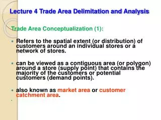
Lecture 4 Trade Area Delimitation and Analysis. Trade Area Conceptualization (1): Refers to the spatial extent (or distribution) of customers around an individual stores or a network of stores.

Lecture 4 Trade Area Delimitation and Analysis
E N D
Presentation Transcript
Lecture 4 Trade Area Delimitation and Analysis Trade Area Conceptualization (1): • Refers to the spatial extent (or distribution) of customers around an individual stores or a network of stores. • can be viewed as a contiguous area (or polygon) around a store (supply point) that contains the majority of the customers or potential customers (demand points). • also known as market area or customer catchment area.
Trade Area Conceptualization (2): • Also viewed as the way of mapping the confines of interaction between a set of store locations and the customers that patronize them. • Interaction can be measured in different ways: number of customers, number of transactions dollar value of transactions • It has a spatial dimension and geographical boundaries, though boundaries are not always clear
Trade Area Conceptualization (3): • Trade Areas vary in size and shape. • Factors that affect trade area size and shape are: • Store size (attractiveness) • Settlement patterns (residential density) • Transportation network • Barriers to movement • Presence of competitors (which provide alternative locations and intervening opportunities) • Can be used to provide information for trade area analysis • characteristics of consumers/customers • screen development potential • assess existing stores performance, • Can be conceptualized and defined in different ways.
Who are concerned with trade area delimitation/analysis? • Retailers/ commercial service providers • Commercial property developers • Real estate department of retail chains • Leasing companies • Location analysts working for the above • Marketing firms who do advertisement for businesses • Educators who train students in the profession of marketing geography, retail geography, and business geography
Three approaches to trade area delimitation: • Spatial Monopoly (Deterministic) • Market Penetration (Probabilistic) • Dispersed Market (Customer profiling)
Deterministic approach has the following characteristics: • Makes a clear-cut assumption about the spatial dimension of the trade area • Trade areas are polygons, each has definite boundaries; they do not overlap • Assumes all customers come from this area; (those living outside are excluded from consideration)
Probabilistic approach has the following characteristics: • Makes no clear-cut assumption about the spatial dimension of the traded areas • Trade areas are not polygons, with no definite boundaries; they overlap • Assign persons (households, CT etc.) to stores partially, with the assumption that people do not always go to the closer store • Treat trade areas as the surface of probabilities: primary (60%) and secondary (60-80%) etc.
Dispersed Market (also known as Customer Profiling) has the following characteristics: • The supplier is often highly specialized. (e.g., specializing one or two lines of imported furniture, selling a narrow selection of books, or serving a widely scattered ethnic group.) • There is no obvious spatial concentration of customers; customers are widely dispersed. • Distance decay relationship is weak • Trade area is defined through customer profiling (i.e., age, income, ethnicity and life style.)
Two types of data for trade area analysis: Secondary data : the most commonly used are census data • less expensive; and need less effort to acquire • can be used to identify potential customers, but many of these potential customers do not necessarily patronize the store. So, the demographic profiles produced are not real customer profile report. Primary data: compiled by retailers. • collected at POS (either based on credit card transactions or by sales associates asking postal codes and phone numbers) • Through customer data analysis, retailers develop a customer profile consisting of demographic, social and economic attributes. • They can also use this profile to search for suitable sites in new markets.
User defined trade area • Also called “rules of thumb”. It is hand-drawn around a given store, from which the analyst believes the majority of customers are attracted. • Relies on the level of experience and expertise of the person who defines the trade area. It assumes that the person has knowledge of customer base and how far they travel. • It is highly subjective, not scientific. • Quality can be improved, if limited customer spotting data are available and used as reference. • Usually used to define trade area for a single store • There are two types of such trade areas: • Unconstrained trade area that do not follow census geographies (but may follow physical barriers) • Boundary constrained
User Defined Trade Area Census tract confined Free-hand FSA confined DA confined
Circular trade area • The easiest, quickest and least expensive method • Trade area defined as a circle using pre-defined radius (usually walking distance or driving distance) • Assuming the transport surface is uniform, and the store is equally accessible from all directions • Competition is not a major factor • Adjacent trade areas may overlap or not overlap, depending on distances between stores and pre-defined radius.
Percentage of Customers • Percentage of customers uses customer data. • The analytical tools is the “customer spotting” map. • This simply is a map of distribution of customers around a given store. • Boundaries are drawn to include the CTs/DAs that contain a given percentage of customers. • Usually, distance is used to select the closest 60% and 80% of the customers to the store location.
Travel Distance/travel time • This method uses travel distance or driving time to define trade area. • can be 5km or 10km. Can also be 20 minutes or 30 minutes. • Distance and travel time are influenced by the characteristics of the road network (such as speed limit, one-way street, number of lanes, road capacity, etc.) • The map may look like a spider’s web • The trade area is irregular shaped
Market Penetration • Divides the area into grids (200x200m, 500x500m, or using DA) • Place the same grid over the customer spotting map • Count the number of spotted customers in each cell • Divide the number of customers in each cell by the cell’s total population • The ratio or percentage is regarded as a measure of market penetration • If sales are known from the customer data, the number of customers can be translated into sales, and sales can be divided by total disposable income in the cell to develop a ratio. • Outward from the store location, the number of cells is counted until 60% or 80% of the customers or sales are reached. These cells form the primary and secondary trade areas. • With this method, there may be some holes which have no data or no customers; or some outliers which have a significant number of customers. It is the analyst’s decision to include them or exclude them.
Thiessen Polygon • a geometric procedure for delimiting theoretical trade areas for a network of stores • assumes the stores are similar in size and sell similar products for similar price; consumers purchase products from the closest store. • most suitable for delimiting trade areas of chain stores.
Statistically-Calculated Probabilistic Method;The Huff Model (1) • Huff model is useful in the following ways: • Generate customer volume estimate for existing stores • Generate customer volume estimate for proposed new stores • Answer such strategic questions: • What would happen to my trade area if my store expand by 50%? • What would happen to my trade area if one of my stores is close? • What would happen to my trade area if an existing competitor were to leave the market? • What if a competitor introduces a new store in the market? • Map the probability surface • Estimate sales potential
Statistically-Calculated Probabilistic Method;The Huff Model (2) Huff model requires the following data: • A list of stores (shopping centers), their locations and attributes (attractiveness) • A list of building block areas (CT or DA) with demographic and social economic data (market size and purchasing power) • A matrix of distance, driving time, travel costs between each building block and each store • A sample data set (for calibrating parameters/weights) .
Statistically-Calculated Probabilistic Method;The Huff Model (3) • The challenge is to estimate the parameters. • There are two ways to estimate them: • To make an ‘educated guess”. This is used when sample data are not available. It depends on the experience and knowledge of the local market. Usually several guesses are made for experiment to find out which one generates better results. • To statistically estimate or calibrate the model. Often, it includes using a number of different non-linear models. This requires the use of sample data. Several parameters are experimented, and a measure of goodness of fit is produced. Calculations are undertaken to estimate the direction and amounts each of the parameters should change to improve the fit. Each change is then entered into the model, and the model is re-run until the best values that give rise to the best fit to the sample data are found.
Sales potential estimate S. P. = No. of HH * average HH income * % of income spent on consumer goods * probability Example: S.P. in building 1 at supermarket A: =567 * $26,700 * 0.3 * 0.93 =$4.22 million