Image Processing 101 - eBook
E N D
Presentation Transcript
Image Processing 101 CHAPTER 1.1 What is an Image? Image processing and computer vision are hot trends in computer science that continue to show strong signs of momentum into the future due to their wide application and optimistic development prospects. In the first post of this blog series, we introduce the fundamentals of image processing by looking at what are images and how images are stored. Digital images can be displayed and processed on a computer and can be divided into two broad categories based on their characteristics – bitmaps and vector images. Bitmaps are based on pixel patterns that are usually represented by a digital array. BMP, PNG, JPG, and GIF are bitmaps. Vector images an infinitely scalable and do not have any pixels since they use mathemati- cal formulas to draw lines and curves. A bitmap image of size M × N is composed of finite elements of M rows and N columns. Each element has a specific position and amplitude, representing the information at the position, such as grayscale and color. These elements are called image elements or pixels, if you want to read about it check outfifthgeek.com. Dynamsoft Corporation | Power Your Development with Enterprise-grade SDKs 2 ph: 1-604-605-5491 | toll: 1-877-605-5491 | e: support@dynamsoft.com
Image Processing 101 Color Space 3. RGB Image Depending on the information represented by each pixel, images can be divided into binary images, grayscale images, RGB images, and index images, etc. In RGB or color, images, the information for each pixel requires a tuple of numbers to represent. So we need a three-dimensional matrix to represent an image. Almost all colors in nature can be composed of three colors: red (R), green (G), and blue (B). So each pixel can be represented by a red/green/blue tuple in an RGB image. 1. Binary Image In a binary image, the pixel value is represented by a 0 or 1. Generally, 0 is for black and 1 is for white. 2. Grayscale Image 4. Indexed Image The grayscale image adds a color depth between black and white in the binary image to form a grayscale image. Such images are usually displayed as grayscales from the dark- est black to the brightest white, and each color depth is called a grayscale, usually denoted by L. In grayscale images, pixels can take integer values between 0 and L-1. An indexed image consists of a colormap matrix, which uses direct mapping of pixel values in an array to colormap values. The color of each pixel in an image is determined by using the corre- sponding value. We discuss this in more detail below. Dynamsoft Corporation | Power Your Development with Enterprise-grade SDKs 3 ph: 1-604-605-5491 | toll: 1-877-605-5491 | e: support@dynamsoft.com
Image Processing 101 How an Image is Stored in Memory The x86 hardware does not have an addressing mode that accesses elements of multi-dimensional arrays. When loading an image into memory space, the multi-di- mensional object is converted into a one-dimensional array. Row major ordering or column major ordering are commonly used. Row Major Ordering C/C++ and Python employ row-major ordering. It starts with the first row and then concatenates the second row to its end, then the third row, etc. This means that in a row-major layout, the last index is the fastest changing. In the case of matrices, the last index is columns. For grayscale images, we can use a matrix to represent the level of gray at each pixel. Take a 4*4 image for example. Pixels by row and column: [0,0] [0,1] [0,2] [0,3] [1,0] [1,1] [1,2] [1,3] [2,0] [2,1] [2,2] [2,3] [3,0] [3,1] [3,2] [3,3] Dynamsoft Corporation | Power Your Development with Enterprise-grade SDKs 4 ph: 1-604-605-5491 | toll: 1-877-605-5491 | e: support@dynamsoft.com
Image Processing 101 Memory: Memory: [0,0] [0,1] [0,2] [0,3] [1,0] [1,1] [1,2] [1,3] [2,0] [2,1] [2,2] [2,3] [3,0] [3,1] [3,2] [3,3] For color images, we need multi-dimensional arrays to store the image information. Dynamsoft Corporation | Power Your Development with Enterprise-grade SDKs 5 ph: 1-604-605-5491 | toll: 1-877-605-5491 | e: support@dynamsoft.com
Image Processing 101 Column-Major Ordering: In the row-major layout of multi-dimensional arrays, the first index is the fastest changing. Below is an example. With the row-major order, the consecutive memory address will be allocated like this: With the column-major order, the consecutive memory address will be allocated like this: Address Access Address Access Image A with 6 pixels: 0 A[0][0] 0 A[0][0] A[0][0] A[0][1] A[0][2] 1 A[1][0] 1 A[0][1] A[1][0] A[1][1] A[1][2] 2 A[0][1] 2 A[0][2] 3 A[1][1] 3 A[1][0] 4 A[0][2] 4 A[1][1] 5 A[1][2] 5 A[1][2] How an Image is Stored in Files True Color (24-bit) 24-bit images commonly use 8 bits of each of R, G, and B. For each of the three primary colors, like grayscale, L levels can be used to indicate how much of this color component is present. For example, for a red color with 256 levels, 0 means no red color and 255 means 100% red. Similarly, green and blue can be divided into 256 levels. Each primary color can be represented by an 8-bit binary data, so the total of 3 primary colors requires 24 bits. The uncompressed raw BMP file is an RGB image stored using the RGB standard. Dynamsoft Corporation | Power Your Development with Enterprise-grade SDKs 6 ph: 1-604-605-5491 | toll: 1-877-605-5491 | e: support@dynamsoft.com
Image Processing 101 Indexed Color For a color image with a height and width of 200 pixels and 16 colors, each pixel is represented by three components of RGB. Thus each pixel is represented by 3 bytes and the entire image is 200 × 200 × 3 = 120KB. Since there are only 16 colors in the color image, you can save the RGB values of these 16 colors with a color table (a 16 × 3 two-dimensional array). We discuss this in further detail below. Every element in the array represents a color, indexed by its position within the array. The image pixels do not contain the full specification of its color, but only its index in the table. For example, if the third element in the color table is 0xAA1111, then all pixels with a color of 0xAA1111 can be represented by “2” (the color table index subscript starts at 0). This way, each pixel requires only 4 bits (0.5 bytes), so the entire image can be stored at 200 × 200 × 0. 5 = 20 KB. The color table referred to above is the palette, which is also often called Look Up Table (LUT). GIF is the most representative image file format that supports indexed color modes. Click here to view the GIF Dynamsoft Corporation | Power Your Development with Enterprise-grade SDKs 7 ph: 1-604-605-5491 | toll: 1-877-605-5491 | e: support@dynamsoft.com
Image Processing 101 Color Models? CHAPTER 1.2 What is a Color Model? A color model is an abstract mathematical model that describes how colors can be represented as a set of numbers (e.g., a triple in RGB or a quad in CMYK). Color models can usually be described using a coordinate system, and each color in the system is represented by a single point in the coordinate space. For a given color model, to interpret a tuple or quad as a color, we can define a set of rules and definitions used to accurately calibrate and generate colors, i.e. a mapping function. A color space identifies a specific combination of color models and mapping functions. Identifying the color space automatically identifies the associated color model. For example, Adobe RGB and sRGB are two different color spaces, both based on the RGB color model. RGB RGB color model stores individual values for red, green, and blue. With a color space based on the RGB color model, the three primaries are added together to create colors from completely white to completely black. Dynamsoft Corporation | Power Your Development with Enterprise-grade SDKs 8 ph: 1-604-605-5491 | toll: 1-877-605-5491 | e: support@dynamsoft.com
Image Processing 101 The RGB color space is associated with the device. Thus, different scanners get different color image data when scanning the same image; different monitors have different color display results when rendering the same image. There are many different RGB color spaces derived from this color model, standard RGB (sRGB) is a popular example. HSV HSV (hue, saturation, value), also known as HSB (hue, saturation, brightness), is often used by artists because it is often more natural to think about a color in terms of hue and saturation than in terms of additive or subtractive color components. The system is closer to people’s experience and perception of color than RGB. In painting terms, hue, saturation, and values are expressed in terms of color, shading, and toning. Dynamsoft Corporation | Power Your Development with Enterprise-grade SDKs 9 ph: 1-604-605-5491 | toll: 1-877-605-5491 | e: support@dynamsoft.com
Image Processing 101 The HSV model space can be described by an inverted hexagonal pyramid. The top surface is a regular hexagon, showing the change in hue in the H direction, from 0 ° to 360 ° is the entire spectrum of visible light. The six corners of the hexagon represent the positions of the six colors of red, yellow, green, cyan, blue, and magenta, each of which is 60 ° apart. The saturation S is represented by the S direction from the center to the hexagonal boundary, and the value varies from 0 to 1. The closer to the hexagonal boundary, the higher the color saturation. The color of the hexagonal boundary is the most saturated, ie S = 1; the color saturation at the center of the hexagon is 0, ie S = 0. The height of the hexagonal pyramid (also known as the central axis) is denoted by V, which represents a black to white gradation from bottom to top. The bottom of V is black, V = 0; the top of V is white, V = 1. Dynamsoft Corporation | Power Your Development with Enterprise-grade SDKs 10 ph: 1-604-605-5491 | toll: 1-877-605-5491 | e: support@dynamsoft.com
Image Processing 101 YUV The Y′UV model defines a color space in terms of one luma component (Y′) and two chrominance (UV) components. The Y′ channel saves black and white data. If there is only the Y component and there are no U and V components, then the graph represented is grayscale. The Y component can be calculated with the following equation: Y = 0. 299*R+ 0. 587*G+ 0. 114*B, which is the commonly used grayscale formula. The color difference U and V are compressed by B-Y and R-Y in different proportions. Compared with RGB, Y’UV does not necessarily store a triple tuple for each pixel. Y′UV images can be sampled in several different ways. For example, with YUV420, it saves one luma component for every point and two chroma values—a Cr (U) value and a Cb (V) value—every 2×2 points. I.E. 6 bytes per 4 pixels. Dynamsoft Corporation | Power Your Development with Enterprise-grade SDKs 11 ph: 1-604-605-5491 | toll: 1-877-605-5491 | e: support@dynamsoft.com
Image Processing 101 The scope of the terms Y′UV, YUV, YCbCr, YPbPr, etc., is sometimes ambiguous and overlapping. Historically, the terms YUV and Y′UV were used for a specific analog encoding of color information in television systems, while YCbCr was used for digital encoding of color information suited for video and still-image compression and transmission such as MPEG and JPEG. Today, the term YUV is commonly used in the computer industry to describe file-formats that are encoded using YCbCr. Reference:Wikipedia Dynamsoft Corporation | Power Your Development with Enterprise-grade SDKs 12 ph: 1-604-605-5491 | toll: 1-877-605-5491 | e: support@dynamsoft.com
Image Processing 101 CHAPTER 1.3 Color Space Conversion In the last post, we discussed a few common color models, specifically RGB, HSV, and YUV. A color model is an abstract mathematical model that describes how colors can be represented as a set of numbers. In this post, we will look at how to convert them to grayscale. Grayscale is a range of gray shades from white to black, as used in a monochrome display or printout. Grayscale images are most commonly used in image processing because smaller data enables developers to do more complex operations in a shorter time. Dynamsoft Corporation | Power Your Development with Enterprise-grade SDKs 13 ph: 1-604-605-5491 | toll: 1-877-605-5491 | e: support@dynamsoft.com
Image Processing 101 Color to Grayscale Conversion 1. RGB to Grayscale There are a number of commonly used methods to convert an RGB image to a grayscale image such as average method and weighted method. Dynamsoft Corporation | Power Your Development with Enterprise-grade SDKs 14 ph: 1-604-605-5491 | toll: 1-877-605-5491 | e: support@dynamsoft.com
Image Processing 101 1.1 Average Method The Average method takes the average value of R, G, and B as the grayscale value. Grayscale = (R + G + B ) / 3. Theoretically, the formula is 100% correct. But when writing code, you may encounter uint8 overflow error — the sum of R, G, and B is greater than 255. To avoid the excep- tion, R, G, and B should be calculated respectively. Grayscale = R / 3 + G / 3 + B / 3. The average method is simple but doesn’t work as well as expected. The reason being that human eyeballs react differently to RGB. Eyes are most sensitive to green light, less sensitive to red light, and the least sensitive to blue light. Therefore, the three colors should have different weights in the distribution. That brings us to the weighted method. 1.2 The Weighted Method The weighted method, also called luminosity method, weighs red, green and blue according to their wavelengths. The improved formula is as follows: Grayscale = 0.299R + 0.587G + 0.114B Dynamsoft Corporation | Power Your Development with Enterprise-grade SDKs 15 ph: 1-604-605-5491 | toll: 1-877-605-5491 | e: support@dynamsoft.com
Image Processing 101 2. YUV to Grayscale YUV is a color encoding system used for analog television. The YUV color model represents the human perception of color more closely than the standard RGB model used in computer graphics hardware and is more size-efficient. 2.1 RGB to YUV Conversion Y = 0.299R + 0.587G + 0.114B U’= (B-Y)*0.565 V’= (R-Y)*0.713 2.2 The Grayscale Value The formula for converting RGB to Y is the same as the formula for converting RGB to grayscale. Therefore: Grayscale = Y 3. HSV to Grayscale HSV (hue, saturation, value) and HSL (hue, saturation, lightness or luminance) are transformations of a Cartesian RGB color space. To convert HSV to grayscale, we first need to convert HSV to RGB and then convert the RGB triple to a grayscale value. Dynamsoft Corporation | Power Your Development with Enterprise-grade SDKs 16 ph: 1-604-605-5491 | toll: 1-877-605-5491 | e: support@dynamsoft.com
Image Processing 101 3.1 HSV to RGB conversion When 0 ≤ H < 360, 0 ≤ S ≤ 1 and 0 ≤ V ≤ 1: C = V × S X = C × (1 – |(H / 60°) mod 2 – 1|) m = V – C (R,G,B) = ((R‘+m)×255, (G‘+m)×255, (B‘+m)×255) 3.2 The Grayscale Value Grayscale = 0.299R + 0.587G + 0.114B Dynamsoft Corporation | Power Your Development with Enterprise-grade SDKs 17 ph: 1-604-605-5491 | toll: 1-877-605-5491 | e: support@dynamsoft.com
Image Processing 101 Binarization: Grayscale to black/white Conversion Binarization converts a grayscale image to a black/white image. This transformation is useful in detecting blobs and further reduces the computational complexity. The critical task is to find a suitable threshold. There are two main methods: Local thresholding Calculates the threshold pixel by pixel Global thresholding Calculates the threshold once for all pixels The images below show an example of before and after binarization. 1. Local Thresholding Method With local thresholding method, a threshold is calculated at each pixel, which depends on some local statistics such as mean, range, and the variance of the pixel neighborhood. The image is divided into several sub-blocks and the distribution of gray-value in each block was analyzed. Dynamsoft Corporation | Power Your Development with Enterprise-grade SDKs 18 ph: 1-604-605-5491 | toll: 1-877-605-5491 | e: support@dynamsoft.com
Image Processing 101 2. Global Thresholding Method The global thresholding method take advantage of the image histogram. The image histogram is a type of statistical graph with grayscale value on the x-axis and the number of pixels for each grayscale on the y-axis. Dynamsoft Corporation | Power Your Development with Enterprise-grade SDKs 19 ph: 1-604-605-5491 | toll: 1-877-605-5491 | e: support@dynamsoft.com
Image Processing 101 Image histogram can be used to automatically determine the value of the threshold to be used for converting a grayscale image to a binary image. The basic idea is to find a point between the peak of the foreground pixel values and the peak of the background pixel values. If the intensity level of a pixel is smaller than the threshold, the pixel is set to black (grayscale = 0), otherwise, it is set to white (grayscale = 255). The threshold serves as a dividing line. Dynamsoft Corporation | Power Your Development with Enterprise-grade SDKs 20 ph: 1-604-605-5491 | toll: 1-877-605-5491 | e: support@dynamsoft.com
Image Processing 101 CHAPTER 2.1 Point Operations Spatial domain image enhancement techniques can be divided into two broad categories: Point operations Neighborhood operations This post discusses the point operations and the next post will be covering the neighborhood operations. Point operations refer to running the same conversion operation for each pixel in a grayscale image. The transformation is based on the original pixel and is independent of its location or neighboring pixels. Let “r” and “s” be the gray value at a point (x, y) of the input image f (x, y) and the output image g (x, y), then the point operation can be defined by the following formula. s= T (r) Where T is the point operator of a certain gray-level mapping relationship between the original image and the output image. Point operations are often used to change the grayscale range and distribution. Dynamsoft Corporation | Power Your Development with Enterprise-grade SDKs 21 ph: 1-604-605-5491 | toll: 1-877-605-5491 | e: support@dynamsoft.com
Image Processing 101 Power-Law (Gamma) Transformation The gamma transform, also known as exponential transformation or power transformation, is a commonly used grayscale non-linear transformation. The mathematical expression of the gamma transformation is as follows: Where x and y are the intensity level of a pixel in input and output, “esp” is the compensa- tion coefficient, and γ is the gamma coefficient. When performing the conversion, it is a common practice to first convert the intensity level from the range of 0 to 255 to 0 to 1. Then perform the gamma conversion and at last restore to the original range. When setting esp = 1, we can get a mapping form like the following, with the gray intensity of the input in the horizontal axis and the gray intensity of the output on the vertical axis. Dynamsoft Corporation | Power Your Development with Enterprise-grade SDKs 22 ph: 1-604-605-5491 | toll: 1-877-605-5491 | e: support@dynamsoft.com
Image Processing 101 Plots of the equation [formula] for various values of γ (c = 1 in all cases). All curves were scaled to fit in the range shown. x-axis represents Input intensity level, r and y-axis represents the output Intensity Level S The gamma transformation can selectively enhance the contrast of the dark region or the light region depending on the value of γ. When γ > 1, the contrast of the light gray area is enhanced. Take γ = 25 for example, the pixels with the range of 0.8-1 (at the scale of 256, it corresponds to 240-255) are mapped to the range of 0-1 When γ < 1, the contrast of the dark gray area is enhanced When γ = 1, this transformation is linear, that is, the original image is not changed Grayscale Threshold Transform Grayscale Threshold Transform converts a grayscale image into a black and white binary image. The user specifies a value that acts as a dividing line. If the gray value of a pixel is smaller than the dividing, the intensity of the pixel is set to 0, otherwise it’s set to 255. The value of the dividing line is called the threshold. The grayscale threshold transform is often referred to as thresholding, or binarization. Dynamsoft Corporation | Power Your Development with Enterprise-grade SDKs 23 ph: 1-604-605-5491 | toll: 1-877-605-5491 | e: support@dynamsoft.com
Image Processing 101 Contrast-Stretching Transformation The goal of the contrast-stretching transformation is to enhance the contrast between different parts of an image, that is, enhances the gray contrast for areas of interest, and suppresses the gray contrast for areas that are not of interest. Below are two possible functions: Dynamsoft Corporation | Power Your Development with Enterprise-grade SDKs 24 ph: 1-604-605-5491 | toll: 1-877-605-5491 | e: support@dynamsoft.com
Image Processing 101 If T(r) has the form as shown in the figure above, the effect of applying the transformation to every pixel to generate the corresponding pixels produce higher contrast than the original image, by: Darkening the levels below k in the original image Brightening the levels above k in the original image Points (r1, s1) and (r2, s2) control the shape of the transformation. The selection of control points depends upon the types of image and varies from one image to another image. If r1 = s1 and r2 = s2 then the transformation is linear and this doesn’t affect the image. In other case we can calculate the intensity of output pixel, provided intensity of input pixel is x, as follows: For 0 <= x <= r1 output = s1 / r1 * x For r1 < x <= r2 output = ((s2 – s1)/(r2 – r1))*(x – r1) + s1 For r2 < x <= L-1 output = ((L-1 – s2)/(L-1 – r2))*(x – r2) + s2 image Dynamsoft Corporation | Power Your Development with Enterprise-grade SDKs 25 ph: 1-604-605-5491 | toll: 1-877-605-5491 | e: support@dynamsoft.com
Image Processing 101 Histogram Equalization Histogram equalization, also known as grayscale equalization, is a practical histo- gram correction technique. It refers to the transformation where an output image has approximately the same number of pixels at each gray level, i.e., the histogram of the output is uniformly distributed. In the equalized image, the pixels will occupy as many gray levels as possible and be evenly distributed. Therefore, such image has a higher contrast ratio and a larger dynamic range. Dynamsoft Corporation | Power Your Development with Enterprise-grade SDKs 26 ph: 1-604-605-5491 | toll: 1-877-605-5491 | e: support@dynamsoft.com
Image Processing 101 CHAPTER 2.2 Image Enhancement What is Image Enhancement? Image enhancement refers to the process of highlighting certain information of an image, as well as weakening or removing any unnecessary information according to specific needs. For example, eliminating noise, revealing blurred details, and adjusting levels to highlight features of an image. Image enhancement techniques can be divided into two broad categories: Spatial domain Frequency domain enhancement the image space that divides an image into uniform pixels according to the spatial coordinates with a certain resolution. The spatial domain methods perform operations on pixels directly enhancement obtained by applying the Fourier Transform to the spatial domain. In the frequency domain, pixels are operated in groups as well as indirectly. Dynamsoft Corporation | Power Your Development with Enterprise-grade SDKs 27 ph: 1-604-605-5491 | toll: 1-877-605-5491 | e: support@dynamsoft.com
Image Processing 101 Image Enhancement Techniques This section discusses the image enhancement techniques implemented in the spatial domain. The concept is to map every pixel onto a new image with a predefined transformation function. g(x, y) = T(f(x, y)) g (x, y) is the output image T is an operator f (x, y) is the input image Image source: Slideshare.net The figure shows a 3 x 3 neighborhood (or spatial filter) of the point (x, y) in an image spatial domain. Moving the neighborhood from pixel to pixel (a procedure called spatial filtering) can generate a new image. Dynamsoft Corporation | Power Your Development with Enterprise-grade SDKs 28 ph: 1-604-605-5491 | toll: 1-877-605-5491 | e: support@dynamsoft.com
Image Processing 101 Basic Intensity Transformation Functions The simplest image enhancement method is to use a 1 x 1 neighborhood size. In this case, the output pixel only depends on the input pixel and the function can be simplified as: s = T(r) Different transformation functions work for different scenarios. Image source: Slideshare.net Dynamsoft Corporation | Power Your Development with Enterprise-grade SDKs 29 ph: 1-604-605-5491 | toll: 1-877-605-5491 | e: support@dynamsoft.com
Image Processing 101 1. Linear Linear transformations include identity transformation and negative transformation. In identity transformation, the input image is the same as the output image. s = r The negative transformation is: s = L – 1 – r = 256 – 1 – r = 255 – r This kind of transformation is suited for enhancing white or gray detail embedded in dark areas of an image. For example, analyzing the breast tissue in a digital mammogram. Image source: Slideshare.net Dynamsoft Corporation | Power Your Development with Enterprise-grade SDKs 30 ph: 1-604-605-5491 | toll: 1-877-605-5491 | e: support@dynamsoft.com
Image Processing 101 2. Logarithmic The equation of general log transformation is: s = clog(1 + r) c is a constant In the log transformation, the low intensity values are mapped into higher intensity values. Image source: Slideshare.net The inverse log transform is opposite to log transform. 3. Power-Law Power-law transformation equation is: Dynamsoft Corporation | Power Your Development with Enterprise-grade SDKs 31 ph: 1-604-605-5491 | toll: 1-877-605-5491 | e: support@dynamsoft.com
Image Processing 101 Comparing to log transformation, gamma transformation can generate a family of possible transformation curves by varying the gamma value. Here are the enhanced images output by using different values. Image source: Slideshare.net Gamma 8 Gamma 10 Gamma 6 Image source: TutorialsPoint.com Dynamsoft Corporation | Power Your Development with Enterprise-grade SDKs 32 ph: 1-604-605-5491 | toll: 1-877-605-5491 | e: support@dynamsoft.com
Image Processing 101 4. Histogram Equalization This method is to boost the global contrast of an image to make it look more visible. The general histogram equalization formula is: CDF refers to the cumulative distribution function L is the maximum intensity value (typically 256) M is the image width and N is the image height h (v) is the equalized value Before Histogram Equalization After Histogram Equalization Image source: Wikipedia Dynamsoft Corporation | Power Your Development with Enterprise-grade SDKs 33 ph: 1-604-605-5491 | toll: 1-877-605-5491 | e: support@dynamsoft.com
Image Processing 101 CHAPTER 2.3 Spatial Filters In the chapter 2.1, we discussed gamma transformation, histogram equalization, and other image enhancement techniques. The commonality of these methods is that the transforma- tion is directly related to the pixel gray value, independent of the neighborhood in which the pixel is located. In this post, we take a look at the spatial domain enhancement where neighborhood pixels are also used. A General Concept The spatial domain enhancement is based on pixels in a small range (neighbor). This means the transformed intensity is determined by the gray values of those points within the neighborhood, and thus the spatial domain enhancement is also called neighborhood operation or neighborhood processing. A digital image can be viewed as a two-dimensional function f (x, y), and the x-y plane indicates spatial position information, called the spatial domain. The filtering operation based on the x-y space neighborhood is called spatial domain filtering. Dynamsoft Corporation | Power Your Development with Enterprise-grade SDKs 34 ph: 1-604-605-5491 | toll: 1-877-605-5491 | e: support@dynamsoft.com
Image Processing 101 The filtering process is to move the filter point-by-point in the image function f (x, y) so that the center of the filter coincides with the point (x, y). At each point (x, y), the filter’s response is calculated based on the specific content of the filter and through a pre- defined relationship called template. If the pixel in the neighborhood is calculated as a linear operation, it is also called linear spatial domain filtering, otherwise, it’s called nonlinear spatial domain filtering. Figure 2.3.1 shows the process of spatial filtering with a 3 × 3 template (also known as a filter, kernel, or window). Dynamsoft Corporation | Power Your Development with Enterprise-grade SDKs 35 ph: 1-604-605-5491 | toll: 1-877-605-5491 | e: support@dynamsoft.com
Image Processing 101 Figure 2.3.1 The coefficients of the filter in linear spatial filtering give a weighting pattern. For example, for Figure 2.3.1, the response R to the template is: R = w(-1, -1) f (x-1, y-1) + w(-1, 0) f (x-1, y) + …+ w( 0, 0) f (x, y) +…+ w(1, 0) f (x+1, y) + w (1, 1) f( x+1, y+1) For a filter with a size of (2a+1, 2b+1), the output response can be calculated with the following function: Smoothing Filters Image smoothing is a digital image processing technique that reduces and suppresses image noises. In the spatial domain, neighborhood averaging can generally be used to achieve the purpose of smoothing. 1. Average Smoothing First, let’s take a look at the smoothing filter at its simplest form — average template and its implementation. Dynamsoft Corporation | Power Your Development with Enterprise-grade SDKs 36 ph: 1-604-605-5491 | toll: 1-877-605-5491 | e: support@dynamsoft.com
Image Processing 101 The points in the 3 × 3 neighborhood centered on the point (x, y) are altogether involved in determining the (x, y) point pixel in the new image “g”. All coefficients being 1 means that they contribute the same (weight) in the process of calculating the g(x, y) value. The last coefficient, 1/9, is to ensure that the sum of the entire template elements is 1. This keeps the new image in the same grayscale range as the original image (e.g., [0, 255]). Such a “w” is called an average template. How it works? In general, the intensity values of adjacent pixels are similar, and the noise causes grayscale jumps at noise points. However, it is reasonable to assume that occasional noises do not change the local continuity of an image. Take the image below for example, there are two dark points in the bright area. Dynamsoft Corporation | Power Your Development with Enterprise-grade SDKs 37 ph: 1-604-605-5491 | toll: 1-877-605-5491 | e: support@dynamsoft.com
Image Processing 101 For the borders, we can add a padding using the “replicate” approach. When smooth- ing the image with a 3×3 average template, the resulting image is the following. The two noises are replaced with the average of their surrounding points. The process of reducing the influence of noise is called smoothing or blurring. 2. Gaussian Smoothing The average smoothing treats the same to all the pixels in the neighborhood. In order to reduce the blur in the smoothing process and obtain a more natural smoothing effect, it is natural to think to increase the weight of the template center point and reduce the weight of distant points. So that the new center point intensity is closer to its nearest neighbors. The Gaussian template is based on such consideration. Dynamsoft Corporation | Power Your Development with Enterprise-grade SDKs 38 ph: 1-604-605-5491 | toll: 1-877-605-5491 | e: support@dynamsoft.com
Image Processing 101 The commonly used 3 × 3 Gaussian template is shown below. 3. Adaptive Smoothing The average template blurs the image while eliminating the noise. Gaussian template does a better job, but the blurring is still inevitable as it’s rooted in the mechanism. A more desir- able way is selective smoothing, that is, smoothing only in the noise area, and not smooth- ing in the noise-free area. This way potentially minimizes the influence of the blur. It is called adaptive filtering. So how to determine if the local area needs to be smoothed with noise? The answer lies in the nature of the noise, that is, the local continuity. The presence of noise causes a grayscale jump at the noise point, thus making a large grayscale span. Therefore, one of the following two can be used as the criterion: Dynamsoft Corporation | Power Your Development with Enterprise-grade SDKs 39 ph: 1-604-605-5491 | toll: 1-877-605-5491 | e: support@dynamsoft.com
Image Processing 101 The difference between the maximum intensity and the minimum intensity of a local area is greater than a certain threshold T, ie: max(R) – min(R) > T, where R represents the local area. The variance is greater than a certain threshold T, ie: D(R) > T, where D(R) represents the variance of the pixels in the area R. 4. Others There are some other approaches to tackle the smoothing, such as median filter and adaptive median filter. Sharpening Filters Image sharpening filters highlight edges by removing blur. It enhances the grayscale transition of an image, which is the opposite of image smoothing. The arithmetic operators of smoothing and sharpening also testifies the fact. While linear smoothing is based on the weighted summation or integral operation on the neighborhood, the sharpening is based on the derivative (gradient) or finite difference. Dynamsoft Corporation | Power Your Development with Enterprise-grade SDKs 40 ph: 1-604-605-5491 | toll: 1-877-605-5491 | e: support@dynamsoft.com
Image Processing 101 How to distinguish noises and edges still matters in sharpening. The difference is that, in smoothing we try to smooth noise and ignore edges and in sharpening we try to enhance edges and ignore noise. Some applications of where sharpening filters are used are: Medical image visualization Photo enhancement Industrial defect detection Autonomous guidance in military systems There are a couple of filters that can be used for sharpening. In this article, we will introduce one of the most popular filters — Laplace operator, which is based on second order differential. The corresponding filter template is as follows: Dynamsoft Corporation | Power Your Development with Enterprise-grade SDKs 41 ph: 1-604-605-5491 | toll: 1-877-605-5491 | e: support@dynamsoft.com
Image Processing 101 With the sharpening enhancement, two numbers with the same absolute value repre- sent the same response, so w1 is equivalent to the following template w2: Taking a further look at the structure of the Laplacian template, we see that the tem- plate is isotropic for a 90-degree rotation. Laplace operator performs well for edges in the horizontal direction and the vertical direction, thus avoiding the hassle of having to filter twice. Example Dynamsoft Corporation | Power Your Development with Enterprise-grade SDKs 42 ph: 1-604-605-5491 | toll: 1-877-605-5491 | e: support@dynamsoft.com
Image Processing 101 Subscribe to our newsletter to learn more about our Image Processing Series. Contact us if you have any questions about Dynamsoft’s enterprise-grade document capture and barcode reading SDKs. Phone support Email support Sales: sales@dynamsoft.com Support: support@dynamsoft.com 1-887-605-5491 (Toll-Free) 1-604-605-5491 About Dynamsoft Corp. Dynamsoft Corp. provides enterprise-class TWAIN™ software development kits (SDK), a Barcode Reader SDK, and a Label Recognition SDK to help developers meet document imaging, scanning, barcode reader, and OCR extraction application requirements when developing web, desktop, or mobile document management and label reading applications. The imaging SDKs help today’s businesses seeking to migrate from wasteful paper-based workflows to efficient paperless electronic document and records management. Thousands of customers use Dynamsoft's solutions. The company also provides enterprise-grade version control software to help developers manage developer teams and projects. Dynamsoft is an associate member of the TWAIN Working Group that develops TWAIN standards. The company was founded in 2003. More information is available at http://www.dynamsoft.com. Dynamsoft Corporation | Power Your Development with Enterprise-grade SDKs 42 ph: 1-604-605-5491 | toll: 1-877-605-5491 | e: support@dynamsoft.com