Download
1 / 36
380 likes | 656 Vues
Decision Analysis (Decision Tables , Utility ). Y. İlker TOPCU , Ph .D. www.ilkertopcu. net www. ilkertopcu .org www. ilkertopcu . info www. facebook .com/ yitopcu twitter .com/ yitopcu. Introduction. One dimensional (single criterion) decision making

E N D
Decision Analysis(Decision Tables, Utility) Y. İlker TOPCU, Ph.D. www.ilkertopcu.net www.ilkertopcu.org www.ilkertopcu.info www.facebook.com/yitopcu twitter.com/yitopcu
Introduction • One dimensional (single criterion) decision making • Single stage vs. multi stage decision making • Decision analysis is an analytical and systematic way to tackle problems • A good decision is based on logic: rational decision maker (DM)
Components of Decision Analysis • A state of nature is an actual event that may occur in the future. • A payoff matrix (decision table) is a means of organizing a decision situation, presenting the payoffs from different decisions/alternatives given the various states of nature.
Basic Steps in Decision Analysis • Clearly define the problem at hand • List the possible alternatives • Identify the possible state of natures • List the payoff (profit/cost) of alternatives with respect to state of natures • Select one of the mathematical decision analysis methods (models) • Apply the method and make your decision
Types of Decision-Making Environments • Type 1: Decision-making under certainty • DMknows with certainty the payoffs of every alternative . • Type 2: Decision-making under uncertainty • DMdoes not know the probabilities of the various states of nature. Actually s/he knows nothing! • Type 3: Decision-making under risk • DMdoes know the probabilities of the variousstates of nature.
Decision Making Under Certainty • Instead of state of natures, a true state is known to the decision maker before s/he has to make decision • The optimal choice is to pick an alternative with the highest payoff
Decision Making Under Uncertainty • Maximax • Maximin • Criterion of Realism • Equally likelihood • Minimax
Maximax Choose the alternative with the maximum optimistic level ok = {oi} = {{vij}}
Maximin Choose the alternative with the maximum security level sk = {si} = {{vij}}
Criterion of Realism Hurwicz suggested to use the optimism-pessimism index (a) Choose the alternative with the maximum weighted average of optimistic and security levels {aoi + (1 – a) si}where 0≤a≤1
Criterion of Realism 120a-20 = 0 a = 0.1667 380a-180 = 120a-20 a = 0.6154 0≤a≤0.1667 “Do nothing” 0.1667 ≤ a ≤ 0.6154 “Construct small plant” 0.6154≤ a ≤ 1 “Construct large plant”
Equally Likelihood Laplace argued that “knowing nothing at all about the true state of nature” is equivalent to “all states having equal probability” Choose the alternative with the maximum row average (expected value)
Minimax Savage defined the regret (opportunity loss) as the difference between • the value resulting from the best action given that state of nature j is the true state and • the value resulting from alternative i with respect to state of nature j Choose the alternative with the minimum worst (maximum) regret
Summary of Example Results METHOD DECISION • Maximax “Construct large plant” • Maximin “Do nothing” • Criterion of Realism depends ona • Equally likelihood “Construct small plant” • Minimax “Construct small plant” The appropriate method is dependent on the personality and philosophy of the DM.
Decision Making Under Risk Probability • Objective • Subjective • Expected (Monetary) Value Expected Value of Perfect Information • Expected Opportunity Loss • Utility Theory Certainty Equivalence Risk Premium
Probability • Aprobabilityis a numerical statement about the likelihood that an event will occur • The probability, P, of any event occurring is greater than or equal to 0 and less than or equal to 1: 0 P(event) 1 • The sum of the simple probabilities for all possible outcomes of an activity must equal 1
Objective Probability P(A) = n(A) / n Determined by experiment or observation: • Probability of heads on coin flip • Probability of spades on drawing card from deck P(A): probability of occurrence of event A n(A): number of times that event A occurs n: number of independent and identical repetitions of the experiments or observations
Subjective Probability • Determined by an estimate based ontheexpert’s • personal belief, • judgment, • experience, and • existingknowledge of a situation
Expected (Monetary) Value Choose the alternative with the maximum weighted row average EV(ai) = vij P(qj)
Sensitivity Analysis EV(Large plant) = $200,000P – $180,000 (1 – P) EV(Small plant) = $100,000P – $20,000(1 – P) EV(Do nothing) = $0P + $0(1 – P)
Sensitivity Analysis Large Plant 250000 Point 2 200000 Small Plant 150000 Point 1 100000 50000 EV 0 0 0.2 0.4 0.6 0.8 1 -50000 -100000 -150000 -200000 P
Expected Value of Perfect Information • A consultant or a further analysis can aid the decision maker by giving exact (perfect) information about the true state: the decision problem is no longer under risk; it will be under certainty. • Is it worthwhile for obtaining perfectly reliable information: is EVPI greater than the fee of the consultant (the cost of the analysis)? • EVPI is the maximum amount a decision maker would pay for additional information
Expected Value of Perfect Information EVPI = EV with perfect information – MaximumEVunder risk EV with perfect information: 200*.6+0*.4=120 Maximum EV under risk: 52 EVPI = 120 – 52 = 68
Expected Opportunity Loss Choose the alternative with the minimum weighted row average of the regret matrix EOL(ai) = rij P(qj)
Utility Theory • Utility assessment mayassign the worst payoff a utility of 0 and the best payoff a utility of 1. • A standard gamble is used to determine utility values: When DM isindifferentbetweentwoalternatives, the utility values of themare equal. • Choose the alternative with the maximum expected utility EU(ai) = u(ai) = u(vij) P(qj)
Standard Gamble for Utility Assessment (p) Best payoff(v*) u(v*) = 1 Lotteryticket (1–p) Worst payoff(v–) u(v–) = 0 Certain money Certainpayoff(v) u(v) = 1*p+0*(1–p)
Utility Assessment (1st approach) (0.5) (0.5) (0.5) x1 u(x1)= 0.5 Best payoff(v*) u(v*) = 1 v* u(v*) = 1 Lottery ticket Lottery ticket Lottery ticket (0.5) (0.5) (0.5) Worst payoff(v–) u(v–) = 0 v– u(v–) = 0 x1 u(x1) = 0.5 x3 u(x3) = 0.25 Certainpayoff(x1) u(x1) = 0.5 x2 u(x2) = 0.75 Certain money Certain money Certain money II I Intheexample: u(-180) = 0 and u(200) = 1 x1= 100 u(100) = 0.5 x2= 175 u(175) = 0.75 x3= 5 u(5) = 0.25 III
Utility Assessment (2nd approach) (p) Best payoff(v*) u(v*) = 1 Lottery ticket (1–p) Worst payoff(v–) u(v–) = 0 Certainpayoff(vij) u(vij) = p Certain money Intheexample: u(-180) = 0 and u(200) = 1 Forvij=–20, p=%70 u(–20) = 0.7 Forvij=0, p=%75 u(0) = 0.75 Forvij=100, p=%90 u(100) = 0.9
Preferences for Risk Riskaversion (avoidance) Risk neutrality (indifference) Utility Riskproness (seeking) Monetary outcome
Certainty Equivalence p X Lottery ticket 1–p Y Certain money Z • If a DM is indifferent between accepting a lottery ticket and accepting a sum of certain money, the monetary sum is the Certainty Equivalent (CE) of the lottery • Z is CE of the lottery (Y>Z>X).
Risk Premium • Risk Premium (RP) of a lottery is the difference between the EV of the lottery and the CE of the lottery • If the DM is risk averse (avoids risk), RP>0 S/he prefers to receive a sum of money equal to expected value of a lottery than to enter the lottery itself • If the DM is risk prone (seeks risk), RP<0 S/he prefers to enter a lottery than to receive a sum of money equal to its expected value • If the DM is risk neutral, RP=0 S/he is indifferent between entering any lottery and receiving a sum of money equal to its expected value