Rules of Differentiation and Their Use in Comparative Statics

1. Rules of Differentiation and Their Use in Comparative Statics • Rules of Differentiation for a Function of One Variables 1. Constant-Function Rule y = f(x) = c, where c is a constant, then = f’(x) = 0

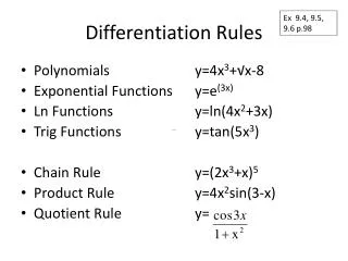
2. Rules of Differentiation 2. Power Function Rule If y=f(x) = xa where a is any real number -<a< = f’(x) = axa-1 Example: If y = f(x) = x-3, then f’(x) = -3x-4 If y = f(x) = , then f’(x) = ½ x-1/2

3. Rules of Differentiation • Rules of Differentiation Involving Two or More Functions of the Same Variable 1. Sum-Difference Rule Example: Short-run total cost, c = Q3-4Q2+10Q+75 MC = = 3Q2-8Q+10

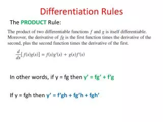
4. Rules of Differentiation 2. Product Rule

5. Findings Marginal Revenue Function from Average Revenue Function Suppose the average revenue (AR) function is specified by AR = 15 – Q Total revenue (TR) = AR x Q = 15Q – Q2 Marginal revenue (MR) = = 15 – 2Q

6. Findings Marginal Revenue Function from Average Revenue Function…… • In general, if AR = f(Q), then TR = AR . Q = Qf(Q), thus MR = = f(Q)+Qf’(Q) Since MR – AR = [f(Q)+Qf’(Q)] – f(Q) = Qf’(Q) they will always differ the amount of Qf’(Q)

7. Findings Marginal Revenue Function from Average Revenue Function…… Also, since AR = If the market is perfect competitive, i.e. the firm takes the price as given, then P = f(Q) = constant. Hence, f’(Q) = 0. Thus, MR – AR = 0 or MR = AR. Under imperfect competition, on the other hand, the AR curve is normally downward sloping, so that f’(Q) < 0. Thus, MR < AR

8. Rules of Differentiation 3. Quotient Rule

9. Relationship between Marginal Cost and Average Cost Functions Given AC = , Q > 0 MC = C’(Q) The rate of change of AC with respect to Q can be found by differentiating AC:

10. Relationship between Marginal Cost and Average Cost Functions…. From this it follows that, for Q > 0

11. Relationship between Marginal Cost and Average Cost Functions…. C MC=3Q2 – 24Q + 60 AC=Q2 – 12Q + 60 Q

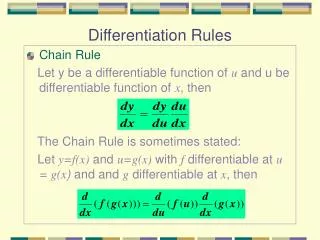
12. Rules of Differentiation 4. Chain Rule If we have a function z = f(y), where y is in turn a function of another variable x, say, y = g(x), then the derivative of z with respect to x is given by Given a x, there must result a corresponding y via the function y = g(x), but this y will in turn being about a z via the function z = f(y)

13. Rules of Differentiation Chain Rule… Example: if z = 3y2 and y = 2x + 5

14. Rules of Differentiation 5. Inverse Function Rule

15. Techniques of Partial Differentiation • Hold the other independent variables constant while allowing one variable to vary Suppose

16. Applications to Comparative-Static Analysis • How the equilibrium value of an endogeneous variable will change when there is a change in any of the exogeneous variables or parameters Market Model For the one-commodity market model Qd = a – bp (a, b > 0) Qs = c + dp (c, d > 0)

17. Applications to Comparative-Static Analysis Market Model …. the equilibrium price and quantity are given by

18. Applications to Comparative-Static Analysis Market Model …. Concentrate on p*, we can get the following 4 partial derivatives

19. Applications to Comparative-Static Analysis Market Model ….

20. Applications to Comparative-Static Analysis • National Income Model Y = C + I0 + G0 (equilibrium condition) C =  + (Y – T) ( > 0; 0 <  < 1) T =  + Y ( > 0; 0 <  < 1) where three endogeneous variables are the national income Y, consumption C, and taxes T.

21. Applications to Comparative-Static Analysis • National Income Model….. The equilibrium income (in reduced form) is

22. Applications to Comparative-Static Analysis • National Income Model….. The government-expenditure multiplier

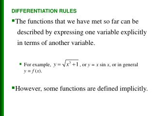
23. Note on Jacobian Determinants • Partial derivatives can also provide a means of testing whether there exists functional (linear or non-linear) dependence among a set of n variables. This is related to the notion of Jacobian determinants

24. Note on Jacobian Determinants… Consider n differentiable functions in n variables not necessary linear y1 = f1(x1, x2,….., xn) y2 = f2(x1, x2,….., xn) …………………….. yn = fn(x1, x2,….., xn) where the symbol fi denotes the ith function, we can derive a total of n2 partial derivatives.

25. Note on Jacobian Determinants… • Arrange the partial derivatives into a square matrix, called a Jacobian matrix and denoted by J, and then take its determinant, the result will be what is known as a Jacobian determinant, J 

26. Jacobian Determinants: Example • Consider two functions • Then the Jacobian is

27. Jacobian Determinants: Theorem • The Jacobian J defined above will be identically zero for values of x1, x2, …xn if and only if the n functions f1, f2,…fn are functionally (linear or nonlinear) dependent. From the above, since J = (24x1 + 36x2) – (24x1 + 36x2) = 0 for all x1 and x2, y1 and y2 are functionally dependent. In fact, y2 is simply y1 squared.