Download
1 / 24
240 likes | 350 Vues
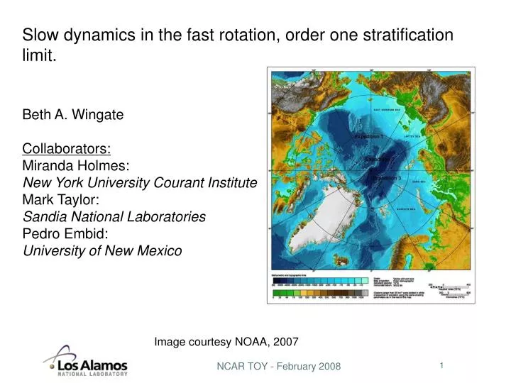
Slow dynamics in the fast rotation, order one stratification limit. Beth A. Wingate Collaborators: Miranda Holmes: New York University Courant Institute Mark Taylor: Sandia National Laboratories Pedro Embid: University of New Mexico. Image courtesy NOAA, 2007.

E N D
Slow dynamics in the fast rotation, order one stratification limit. Beth A. Wingate Collaborators: Miranda Holmes: New York University Courant Institute Mark Taylor: Sandia National Laboratories Pedro Embid: University of New Mexico Image courtesy NOAA, 2007
High rotation rate effects - Taylor Columns • Taylor-Proudman theorem: In rapidly rotating flow, the flow two-dimensionalizes. • Hogg, “On the stratified Taylor Column” JFM, 1973 • Davies, “Experiments on Taylor Columns in Rotating and Stratified Flow, JFM 1971 • Taylor columns have been observed in the high latitudes, and they frequently involve some degree of stratification too. These are called Taylor Caps. See for example Mohn, Bartsch, Meinche Journal of Marine Science, 2002
Triply periodic rotating and stratified Boussinesq equations
Method of Multiple Scale -- Embid and Majda style. To avoid secularity the second order term must be smaller than the leading order term. Embid, P and Majda, A “Low Froude number limiting dynamics for stably stratified flow with small or finite Rossby number.” Geophysical and Astrophysical Fluid Dynamics, 87 pp 1-50
The equations for the slow dynamics are, , u, v, w all functions of (x,y) only. Note change of notation.
Numerical Simulations High wave number white noise forcing. Smith and Waleffe, JFM, 2002 Zonal Velocity
Numerical Simulations High wave number white noise forcing. Smith and Waleffe, JFM, 2002 Zonal Velocity
Numerical simulations - Globally integrated total and slow potential enstrophy. High wave number white noise forcing. Smith and Waleffe, JFM, 2002
Take home message • Following Embid and Majda we use the method of multiple scales and fast wave averaging to find slow dynamics for Rossby to zero, finite Froude limit. • The leading order solution to the stably stratified, triply periodic fast-rotation Boussinesq equations has both fast and slow components. Leading order potential enstrophy is slow. • The slow dynamics evolves independently of the fast. • Equations for the slow dynamics including their conservation laws. Two-D NS and w/theta dynamics. • Preliminary numerical results support the slow conservation laws and the potential enstrophy only slow when Ro is small.
In operator form Embid and Majda, 1996, 1997 Schochet, 1994 Babin, Mahalov, Nicolaenko, 1996
Method of Multiple scales - write the abstract form with epsilon and tau. To lowest order
Method of multiple of time scales The order 1solution is a function of the leading order solution. Duhammel’s formula
Separation of time scales - Fast wave averaging equation Where solves: And therefore, the solution to leading order is And since the fast linear operator is skew-Hermitian, has an orthogonal decomposition into fast and slow components: Using the fact that , the leading order solution looks like,
Separation of time scales - Fast wave averaging equation Therefore, study the solutions of the linear problem:
By direct computation the fast wave averaging equation Compute the evolution equation for the Fourier amplitudes
Example of a linear operator For the linear operators the only contributions from averaging in time are the result of modes with the same frequency and wave number. So they only contribute slow modes to the evolution of the slow mode dynamics.
The nonlinear operator Three wave resonances means we must choose k’ and k’’ such that You can show that the interaction coefficients are zero for the fast-fast interaction. Which means that the slow dynamics evolves independently of the fast.
Find the equations for the slow dynamics Knowing the slow dynamics evolves independently of the fast we can find the equations for the slow dynamics by projecting the solution and the equations onto the null space of the fast operator .Then the fast wave averaged equation for the slow modes becomes,
The leading order conservation laws in the absence of dissipation, Using the same arguments as Embid and Majda, 1997, there is conservation in time of the slow to fast energy ratio. This means the total energy conservation is composed of both slow and fast dynamics. But the leading order potential enstrophy is composed only of the slow dynamics.