Track Fitting ( Kalman Filter)
Track Fitting ( Kalman Filter). Least Squares Fitting. Generally accepted solution: Kalman filter at Gaussian level optimal correction of multiple scattering (“process noise”) energy loss can be incorporated similarly with “smoother”, full information at every point of trajectory

Track Fitting ( Kalman Filter)
E N D
Presentation Transcript
Least Squares Fitting Generally accepted solution: Kalman filter at Gaussian leveloptimal correction of multiple scattering (“process noise”) energy loss can be incorporated similarly with “smoother”, full information at every point of trajectory convenient for matching with other components
What the Kalman filter is • A progressive way of performing a least-squares fit • Mathematically equivalent to the latter What it is not: • a pattern recognition method (though it can be efficiently used within one) • a “robust” fitting method
Information Flow in the Track Fit Origin • Effects influencing the amount of information contained in the measurements • Information that the fit has to take into account Dilution of information Increase of information
Cx-x Cx-s Cs-x Cs-s 1 z(k+1)-z(k) 0 1 KalmanFilter The Kalman filter process is a successive approximation scheme to estimate parameters Simple Example: 2 parameters - intercept and slope: x = x0 + Sx * z; P = (x0 , Sx) Errors on parameters x0 & Sx (covariance matrix): C = Cx-x = <(x-xm)(x-xm)> In general C = <(P - Pm)(P-Pm)T> Propagation: x(k+1) = x(k)+Sx(k)*(z(k+1)-z(k)) Pm(k+1) = F(dz) * P(k) where F(dz) = Pm(k+1) P(k) k+1 Cm(k+1) = F(dz) *C(k) * F(dz)T + Q(k) Noise: Q(k) (Multiple Scattering) k
k+1 Noise (Multiple Scattering) k KalmanFilter Form the weighted average of the k+1 measurement and the propagated track model: Weights given by inverse of Error Matrix: C-1 Pm(k+1) Hit: X(k+1) with errors V(k+1) Cm-1(k+1)*Pm(k+1)+ V-1(k+1)*X(k+1) P(k+1) = and C(k+1) = (Cm-1(k+1) + V-1(k+1))-1 Cm-1(k+1) + V-1(k+1) Now its repeated for the k+2 planes and so - on. This is called FILTERING - each successive step incorporates the knowledge of previous steps as allowed for by the NOISE and the aggregate sum of the previous hits.
KalmanFilter We start the FILTER process at the conversion point BUT… We want the best estimate of the track parameters at the conversion point. Must propagate the influence of all the subsequent Hits backwards to the beginning of the track - Essentially running the FILTER in reverse. This is call the SMOOTHER & the linear algebra is similar. Residuals & c2: Residuals: r(k) = X(k) - Pm(k) Covariance of r(k): Cr(k) = V(k) - C(k) Then: c2 = r(k)TCr(k)-1r(k) for the kth step
How the Kalman Filter Works -- details • Trajectory until point (k-1) point k-1
How the Kalman Filter Works • Trajectory until point (k-1) • Prediction (without process noise) Prediction point k-1
How the Kalman Filter Works Prediction • Trajectory until point (k-1) • Prediction (with process noise = mult. scattering) • Filter point k-1 Filtering of k-th point
How the Kalman Filter Works Multiple scattering Prediction • Trajectory until point (k-1) • Prediction (with process noise = mult. scattering) point k-1
How the Kalman Filter Works Multiple scattering Prediction • Trajectory until point (k-1) • Prediction (with process noise = mult. scattering) • Filter point k-1 Filtering of k-th point
Some Math: Prediction Parameters & covariance matrix at (k-1) Prediction Prediction equations Process noise Transport matrix • Transports the information up to the (k-1)-th hit to the location of the k-th hit • Process noise takes random perturbations into account (e.g. multiple scattering, radiation)
Prediction vs. Measurement Measurement & covariance matrix at (k) Measurement equations Projection matrix Residual • Projection matrixHkconnects parameter vector (e.g. 5D) and the actual measurement (e.g. 1D)
In this formulation (“gain matrix formalism”), the matrix that needs to be inverted has only the dimension of the measurement (here: 1) Some Math: Filter “Gain matrix” Filter equations Filtered parameters & covariance matrix at (k) • In this formulation (“gain matrix formalism”), the matrix that needs to be inverted has only the dimension of the measurement (here: 1)
Along the Trajectory • Traditionally, the Kalman filter proceeds in the direction opposite to the particle’s flight • parameter estimate near point of origin contains information of all hits & is most precise production vertex direction of flight production vertex direction of filter
Along the Trajectory (cont’d) • If precise parameters at both ends are needed, two filters in opposite directions can be combined production vertex direction of filter 1 production vertex direction of filter 2
Along the Trajectory (cont’d) • The orthodox method of propagating the full information to all points of the trajectory is the “Kalman smoother” • Excellent, but computing intensive • one parameter vector size matrix to invert per step production vertex direction of flight production vertex direction of filter direction of smoother
Process Noise & How to Calculate It • Important: multiple scattering model • evaluate contribution to covariance matrix • depends on track model (example is for tx = tan x, ty = tan y) • angular elements of Q (t = thickness in terms of radiation length)
Extended (“thick”) Scatterers • In this case, also the spatial components of the process noise matrix Q are non-zero (l = thickness in terms of radiation length, D=direction)
Nonlinear fit • With non-linear transport or measurement equation, generalizations are necessary • Optimal properties are retained if linear expansion is made in the right places • in general, this requires iteration R. Mankel, Kalman Filter Techniques
Nonlinear fit (cont’d) • Knowledge of derivatives important • for helical tracks, calculate analytically • for a parameterized inhomogeneous field, transport & calculation of derivatives are usually done numerically • e.g. embedded Runge-Kutta method (adaptive step size) • see T. Oest, HERA-B notes 97-165 and 98-001, and A. Spiridonov, HERA-B note 98-133 • In case derivatives depend on parameters, iteration may be needed R. Mankel, Kalman Filter Techniques
Outlier Removal • In least squares fitting, outlier hits have bad influence on the parameter estimate • outliers should be removed • The traditional method of removing outliers is based on the 2 contribution of the hit to the fit • in Kalman filter language: smoothed 2s • Problems: • good hits can have a worse 2 than bad hits nearby that are causing the problem • “digital” decisions may result in bad convergence R. Mankel, Kalman Filter Techniques
Robust Estimation • Least squares fitting (& thereby Kalman filtering) reaches its limits when underlying statistics are far from Gaussian • typical example: 2distributions in presence of multiple scattering • This problem is more pressing in electron fitting with plenty of material radiation • for general treatment, see Stampfer et al, Comp.Phys.Comm. 79, 157 R. Mankel, Kalman Filter Techniques
Kalman Filter & Pattern Recognition • Kalman filter can be used very efficiently at the core of track following methods • “Concurrent track evolution” • “Combinatorial Kalman filter” • within & without magnetic field see for example Nucl. Instr. Meth. A395, 169; Nucl. Instr. Meth. A426, 268 • will not be discussed in detail here R. Mankel, Kalman Filter Techniques
Further Reading • Many excellent papers exist, which unfortunately cannot be done justice by listing them all here • A review of tracking methods with many references to the original literature can be found inR. Mankel, Rep. Prog. Phys. 67 (2004) 553—622 (online at http://stacks.iop.org/RoPP/67/553) R. Mankel, Kalman Filter Techniques
History 1785 Charles Coulomb, 1900 Elster and Geitel Charged body in air becomes discharged – there are ions in the atmosphere 1902 Rutherford, McLennan, Burton: air is traversed by extremely penetrating radiation (g rays excluded later) 1912 Victor Hess Discovery of “Cosmic Radiation” in 5350m balloon flight, 1936 Nobel Prize 1933 Anderson Discovery of the positron in CRs – shared 1936 Nobel Prize with Hess 1933 Sir Arthur Compton Radiation intensity depends on magnetic latitude 1937 Street and Stevenson Discovery of the muon in CRs (207 times heavier than electron) 1938 Pierre Auger and Roland Maze Rays in detectors separated by 20 m (later 200m) arrive simultaneously 1985 Sekido and Elliot very energetic ions impinging on top of atmosphere First correct explanation: “Somewhat” open question today: where do they come from ?
Victor Hess, return from hisdecisive flight 1912 (reached 5350 m !)radiation increase > 2500m
Satellite observations of primaries Primaries: energetic ions of all stable isotopes: ~85% protons, ~12% a particles Similar to solar elemental abundance distribution but differences due to spallation during travel through space (smoothed pattern) Li, Be, or B Cosmic Ray p or a C,N, or O(He in early universe) Major source of 6Li, 9Be, 10B in the Universe (some 7Li, 11B)
NSCL Experiment for Li, Be, and B production by a+a collisions Mercer et al. PRC 63 (2000) 065805 170-600 MeV Identify and count Li,Be,B particles Measure cross section: how many nuclei are made per incident a particle
Ground based observations Space Cosmic Ray (Ion, for example proton) Atmospheric Nucleus Earth’s atmosphere (about 50 secondaries after first collision) p+ p- po po g g p+ p- e+ e- m+ (~4 GeV, ~150/s/cm2) nm e- g Electromagnetic Shower Plus some:Neutrons14C (1965 Libby) Hadronic Shower (on earth mainly muons and neutrinos) (mainly g-rays)
Cosmic ray muons on earth Lifetime: 2.2 ms – then decay into electron and neutrino Travel time from production in atmosphere (~15 km): ~50 mswhy do we see them ? Average energy: ~4 GeV (remember: 1 eV = 1.6e-19 J) Typical intensity: 150 per square meter and second Modulation of intensity with sun activity and atmosphericpressure ~0.1%
Ground based observations Advantage: Can build larger detectors can therefore see rarer cosmic rays Disadvantage: Difficult to learn about primary Observation methods: 1) Particle detectors on earth surface Large area arrays to detect all particles in shower 2) Use Air as detector (Nitrogen fluorescence UV light) Observe fluorescence with telescopes Particles detectable across ~6 kmIntensity drops by factor of 10 ~500m away from core
electrons • -rays muons Atmospheric Showers and their Detection Fly’s Eye technique measures fluorescence emission The shower maximum is given by Xmax~ X0 + X1 log Ep where X0 depends on primary type for given energy Ep Ground array measures lateral distribution Primary energy proportional to density 600m from shower core
Air Shower Physics The actors: Nuclei composed of nucleons N (p,n) Pions: π+, π-, π0 Muons: μ+, μ- Electrons, positrons: e+, e- Gamma rays [photons]: γ The actions: N + N lots of hadronic particles and anti-particles (mostly pions, equal mix of π+,π-,π0) π±+ N lots of hadronic particles and anti-particles (mostly pions, equal mix of π+,π-,π0) π± μ± + ν (decay lifetime is 1/100 muon lifetime) π0 γ + γ immediate decay (10-16 sec) γ e+ + e- (and recoiling nucleus) [“pair production”] e± e± + γ (and recoiling nucleus) [“bremsstrahlung” or “brake radiation”]
Each π0 decay produces two photons (γ’s), which transfers energy from the “hadronic cascade” to the “electromagnetic cascade.” γ Air shower building block: The electromagnetic cascade Pair production and bremsstrahlung In this simplified picture, the particle number doubles in each generation. Each generation takes one radiation length (37 g/cm2 in air). The cascade continues to grow until the average energy per particle is less than an electron loses to ionization in one radiation length (81 MeV). It is then at its maximum “size,” and the number of particles then decreases. e+ e- γ e- e+ γ γ e+ e- e+ e+ e- e- γ
Particle detector arrays Largest, prior to Pierre Auger project: AGASA (Japan) 111 scintillation detectors over 100 km2 Other example: Casa Mia, Utah:
Air Scintillation detector 1981 – 1992: Fly’s Eye, Utah1999 - : HiRes, same site • 2 detector systems for stereo view • 42 and 22 mirrors a 2m diameter • each mirror reflects light into 256 photomultipliers • see’s showers up to 20-30 km height
Pierre Auger Project Combination of both techniques Site: Argentina + ?. Construction started, 18 nations involvedLargest detector ever: 3000 km2,1600 detectors 40 out of 1600 particle detectors setup (30 run)2 out of 26 fluorescence telescopes run
Other planned next generation observatories Idea: observe fluorescence from space to use larger detector volume OWL (NASA)(Orbiting Wide Angle Light Collectors) EUSO(ESA for ISS)(Extreme Universe Space Observatory)
Energies of primary cosmic rays ~E-2.7 Observable bysatellite ~E-3.0 ~E-3.3 ~E-2.7 Lower energiesdo not reach earth(but might get collected) UHECR’s: 40 events > 4e19 eV7 events > 1e20 eVRecord: October 15, 1991Fly’s Eye: 3e20 eV many Joules in one particle! Man made accelerators
Origin of cosmic rays with E < 1018 eV Direction cannot be determined because of deflection in galactic magnetic field M83 spiral galaxy Galactic magnetic field
Precollapse structure of massive star Iron core collapses and triggers supernova explosion