Download
1 / 13
130 likes | 224 Vues
Study on cosmic radiation antiprotons, their production spectrum, and solar modulation using simulation models and experimental data. Antiproton LIS calculated with MSDM model and compared with theoretical approximations.

E N D
Antiprotons of interstellar origin at balloon altitudes: Flux simulations U. B. Jayanthi , K. C. Talavera Instituto Nacional de Pesquisas Espaciais (INPE), Brasil. A. A. Gusev Space Research Institute (IKIRAS), Moscow, Russia. 21st European Cosmic Ray Symposium, Košice, Slovakia, 9-12 September 2008
INTRODUCTION • The interest of antimatter component in the cosmic radiation ranges from the basics of cosmology . • The CR antiprotons are expected as secondary products of the primary CR interactions with the interstellar medium that is supported by observations in experiments (Asaoka, et al., 2002; Boezio, et al., 2000; Grimani, et al., 2002; Wang, et al., 2002). • Continuing simulations are made considering the solar modulation as initiated by Perko (1987) to explain the observational result at ~0.2 GeV of Buffington et al. (1981) which indicated a possible excess at energies <1GeV. • The recent experimental data from different balloon experiments at different solar activity phases, provided a very good opportunity to understand the modulation process as well as the similarity in the proton and antiproton transport, inspite of fluctuations in data and the model approximations.
2 Interstellar antiproton fluxes In our simulation the antiproton LIS Fp (Ep) was obtained through the Leaky-box model as a solution of the integro-differential equation (Ginzburg, 1964): This considers the production of the secondary antiprotons Q2 p~ by CR proton flux Fp(Ep) and the subsequent tertiary antiprotons Q3 p~ , and includes the flux decreases due to escape (λesc) and interaction (λinel), and the energy losses <dE/dx> in the interstellar matter.
2.1 Antiproton production spectrum • The antiproton production spectrumi.e. the source functionQ 2 p~ + Q 3 p~ in Eq.(1) is a sum ofthecontributions from interactions of the protons and antiprotons with the interstellar H, He and O nuclei in the interstellar matter. The corresponding densities nj are 1, 0.1, 8·10-4 cm-3 (Simon, et al., 1998). • The production of antiprotons and antineutrons was simulated with a Multi Stage Dynamical Model (MSDM) Monte Carlo code (Dementyev and Sobolevsky, 1999). The code simulates yield from a nuclear reaction (x,A) of an incident particle x with a target nucleus A. The projectile can be a hadron (n, n ~ , p, p~ ) or a meson (+,-,0, K+, K-, K 0 ) with kinetic energies from 10 MeV up to 1 TeV. The target can be any nucleus with the atomic mass A≥1. The code simulates all the stages of hadron-nucleus and nucleus-nucleus interactions inside the target using the exclusive approach on the basis of models described by Botvina et al. (1997). • The code produces energy spectra and angular distributions of the reaction products together with total and inelastic cross sections and multiplicities.
Fig. 1: Antiproton and antineutron production cross section for p+H reaction. Symbols mark the MSDM results; thick solid lines represents the Tan and Ng (1983) approximation.
Fig. 2. Antiproton and antineutron production cross section of p +H reaction simulated with the MSDM code.
2.2 Antiproton LIS • For our solution, the rigidity (R) dependent escape path length for antiprotons in the Galaxy is from Jones et al. (2000), the interaction length λinel of antiprotons including annihilationis simulated with the MSDM and the stopping power <dE/dx> is calculated utilizing standard procedure(e.g. PSTAR-NIST). The Eq.1 is solved through an iteration procedure using the “Mathematica”package. The solution readily converges in the third iteration.
The MSDM cross section provides about two times larger tertiary output Q3 p~ in the range of 0.3-3 GeV as compared to the uniform distribution. In the energy range of 0.04-2 GeV the LIS obtained with MSDM slightly exceeds that obtained with the Tan and Ng (1983) approximation and the maximum deviations are ≤ 40% at Ep =0.2 GeV Fig. 3. The interstellar secondary antiproton production spectra simulated using the MSDM and Tan&Ng (1983) cross sections.
2.3 Solar modulation of the LIS • The LIS modulation in the heliosphere is considered on the basis of transport equation for the spherically-symmetric case (Gleeson and Axford, 1968; Fisk et al., 1973). The “force field” approximation inherently neglects the heliospheric gradient and curvature drifts but considers the diffusion, convection and adiabatic deceleration:
FHB, EHB, PHB , and F1AU, E1AU, P1AU, are the antiproton flux, total energy in GeV, momentum in GV at heliospheric boundary (HB) and at the Earth’s orbit (1AU) respectively, m0 is the proton rest mass in GeV. V is the average solar wind speedin 103 km/hr. Physical sense of the solution implies a conservation of the distribution function F/P2for particle energy decreases from EHB down to E1AU in travel from heliosphere RHB to the Earth at 1AU. • The heliospheric conditions are described by the “force field” parameter Φ determined by the solar wind speed V and the heliospheric boundary distance RHB. In oursimulation we used A=17, Pc=1.015 GV (Perko, 1987) who showed that for the energies ≥0.02 GeV the Eq.2 approximates the exact solution of the equation of Gleeson and Axford (1968) for the proton spectrum EHB-γ (where =PHB/EHB is the proton speed) and also consistent with the solar flare proton observations. • The Φ magnitude is determined from the best fit approximation with the Eq.2 of the observed proton spectrum F1AU assuming the interstellar spectrum as FHB (EHB) =16470EHB-2.76 protons/m s sr GeV.The fits furnish Φmax=0.964 GeV and Φmin =0.368 GeV corresponding to solar maximum and minimum epochs.
Fig. 4: Simulated LIS and the modulated spectra compared with experimental observations.
The results of our simulated spectrum • In fig 4 .Also antiproton fluxes obtained in different experiments conducted at different solar minimum and maximum periods. The increases in the low energy fluxes are provided by the higher fluxes of more energetic particles enriching the <1 GeV region due to adiabatic energy losses. The steeper the low energy branch of the LIS spectrum the more pronounced is the above mentioned increases (Boella et al., 1998). The results of the simulations provided flux values of ~ 4x10⁻³ to 10-2 and ~ 10-2 to 1.7 x 10⁻² antiprotons/m2 s sr GeV at energies of 0.2 and 1 GeV respectively, corresponding to the solar maximum and minimum epochs. The curve for Φ=1.5 is the lower limit for all the experimental data. It may correspond for example to V = 103 km/hour and RHB=70 AU.
4 Conclusions • A simulation of the expected fluxes of interstellar origin incorporating solar modulation is attempted to explain the recent measurements of antiprotons at solar maximum and minimum in balloon experiments. Particularly for the possible excess of the < 1GeV interstellar antiproton observations, initially the simulation considered the tertiary and antineutron decay antiprotons of the LIS source. The interaction cross sections by the MSDM Monte Carlo code provided a slightly larger antiproton flux in the energy range of 0.1-1 GeV compared to the Tan and Ng (1983) approximation. Then the “force field” solution for the solar modulation with rigidity dependence in compliance with the LIS and the 1AU spectra showed satisfactory agreement between the simulations and the balloon results at the solar maximum and minimum periods..