Download
1 / 11
120 likes | 142 Vues
Explore the impact of money supply on GDP and FX rates, including the Quantity Theory of Money and Monetary Models of FX Rates to forecast exchange rate movements in the short run. Learn how changes in money supply affect exchange rates globally.

E N D
Outline 4: Exchange Rates and Monetary Economics: How Changes in the Money Supply Affect Exchange Rates and Forecasting Exchange Rates in the Short Run 4.1 Introduction 4.2 Quantity Theory of Money 4.3 Monetary Approach to Exchange Rates 4.4 Conclusion
4.1 Introduction Impact of money supply on GDP is the major subject of monetary and macroeconomics. Important Question: Can we manage the economy (dampen business cycles) by changing the money supply. Since FX rates are the prices of one money for another, these “money models” of the economy are applied to different countries to predict and explain future movements in FX rates.
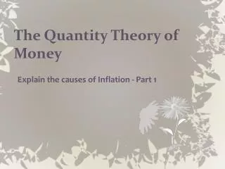
4.2 Quantity Theory of Money (QTM) The QTM is a simple macro model that explains the relationship between inflation, money supply and the level of output (real GDP).
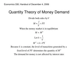
4.2 Quantity Theory of Money The QTM model is: PY = MV Where: P = price level (e.g., consumer price index) Y = sometimes denoted as Q is real GDP M = money supply V = velocity of money or the number of times the average dollar is used in a transaction in a year
4.2 Quantity Theory of Money Assume that V is a constant and divide both sides by Y: If M grows faster than Y, P rises, or if M rises and Y is constant, prices will rise the same as M. Now for the foreign country:
4.2 Quantity Theory of Money PPP shows that: Therefore:
4.2 Quantity Theory of Money QTM shows that, in the long run, relative growth of M versus Y for two countries determines the direction of the FX rate.
4.3 Monetary Model of FX Rates The money market demand equation: md = p + ay – br md depends on the price level (p) national income (y) and interest rates (r), where a and b are slopes that are the same in both countries. All variables are in natural logs or growth rates except for the interest rate, which is already a percentage. Higher price levels requires higher money balances for transactions, higher national income creates a higher demand for money for transactions and higher interest rates lowers demand for money The money supply, “controlled” by the central bank, is ms. Since equilibrium always holds in money market, ms always equals md, therefore: ms = p + ay – br We denote mdand ms as m.
4.3 Monetary Model of FX Rates The foreign country money market equation is the same except variables have a “ * “: m* = p* + ay* – br*, where m = md = ms. Since the FX rate is determined by relative md and ms in both countries for a given income and rate of interest, subtract foreign equation from domestic: m – m* = p – p* + a( y – y*) – b(r – r*)
4.3 Monetary Model of FX Rates Assume that PPP holds continually and E is the dollar price of the foreign currency: or in growth rate form (lower case letters denote growth rate or logs): e = p – p* Substitute e for p – p* in money equation and solve for e: e = (m – m*) – a( y – y*) + b(r – r*)
4.3 Monetary Model of FX Rates e = (m – m*) – a( y – y*) + b(r – r*) If m is increased in the US faster than in the foreign country (m*), holding y and r constant, the $ price of the foreign currency will rise by the difference in m growth. Note that slope on (m – m*) is assumed to be 1.0 by theory. If slope is greater than 1.0, changes in M may be a source of instability on E.