Download
1 / 25
250 likes | 390 Vues
Efficient Discrete-Time Simulations of Continuous-Time Quantum Query Algorithms. Rolando D. Somma Joint work with R. Cleve, D. Gottesman, M. Mosca, D. Yonge-Mallo. QIP 2009 January 14, 2009 Santa Fe, NM. For quantum algorithms, we consider a reversible version of BB:.

E N D
Efficient Discrete-Time Simulations of Continuous-Time Quantum Query Algorithms Rolando D. Somma Joint work with R. Cleve, D. Gottesman, M. Mosca, D. Yonge-Mallo QIP 2009 January 14, 2009 Santa Fe, NM
For quantum algorithms, we consider a reversible version of BB: Query or Oracle Model of Computation Given a black-box (BB) BB Want to learn a property of the N-tuple
Quantum algorithms in the oracle model U1 U2 U3 M M Output gives some property of M … M M M Known unitaries Examples * Shor’s factorization algorithm: Period-finding * Grover’s algorithm: find a marked element * Element Distinctness (Ambainis): finding two equal items Query or Oracle Model of Computation Oracle models are useful to obtain bounds in complexity and to make a fair comparisson between quantum and classical complexities
Continuous-Time Quantum Query Model of Computation Query cost 1- Query Hamiltonian fractional query 2- Time-dependent Driving Hamiltonian (known) 3- Evolution time (or total query cost) T>0 M Output gives some property of M M M M M * E. Farhi and S. Gutmann, Phys. Rev. A 57, 2043 (1998)
Motivations: • Some quantum algorithms have been discovered in the continuous time query model • “Exponential algorithmic speed up by quantum walk”, Childs et. al. • [Proc. 35th ACM Symp. On Th. Comp. (2003)] Given: an oracle for the graph, and the name of the Entrance. Find the name of the Exit.
Motivations: • Some quantum algorithms have been discovered in the continuous time query model • “A Quantum Algorithm for Hamiltonian NAND tree”, Farhi, Goldstone, Gutmann • quant-ph/0702144 N The query Hamiltonian is built from the adjacency matrix of a graph determined by the tree and the input state. It outputs the (binary) NAND in time
Q(1): Is the CT query model more powerful than the conventional query model? The actual implementation of a quantum algorithm in the CT setting may require knowledge on the query Hamiltonian which my not be an available resource. Yes: It has been known(2) that this can be done with cost We present a method to do it at a cost (1) C. Mochon, Hamiltonian Oracles, quant-ph/0602032 (2) D. Berry, G Ahokas, R. Cleve, and B.C. Sanders, Commun. Math. Phys. 270, 359 (2007) Motivations: Is it possible to convert a quantum algorithm in the CT setting to a quantum algorithm in the more conventional query model?
MAIN RESULTS: Theorem: Any continuous-time T-query algorithm can be simulated by a discrete-time O(TlogT)-query algorithm Corollary: Any lower bounds on discrete query complexity carry over to continuous query complexity within a log factor
Quantum Algorithm: Overview The construction has many steps… • • Step 1: Discretization using a (first order) Suzuki-Trotter approximation • •Step 2: Probabilistic simulation of fractional queries using (low-amplitude) • controlled discrete queries • 1 and 2 yield simulations of cost O(T2) • Step 3: Reduction on the amount of discrete queries by disregarding high- • Hamming weight control-qubit states • •Step 4: Correction of errors due to step 2
Step 1: Trotter-Suzuki Approximation U1 U2 U3 M M … M M M Step 1: Fidelity Still p>>T fractional queries Algorithm in the CT setting Output gives some property of M M M M M
Step 1: Trotter-Suzuki Approximation U1 U2 U3 M M … M M M Step 1: Fidelity Still p>>T fractional queries It doesn’t work in general…
Step 2: Probabilistic Simulation of Fractional Queries M R2 R1 Why do we want this conversion? The actual query cost is much lower than p. In step 3, we take advantage of this situation.
Step 2: Probabilistic Simulation of Fractional Queries R1 R2 M R1 R2 M R1 R2 M U1 U2 U3 M M … M M M U1 U2 U3 Up M M … M M M
Step 3: Reducing the amount of queries For a segment of size m, it is likely to succeed There are 4T segments of that size in the total circuit We break the circuit in segments of size m : R1 R2 M … R1 R2 M R1 R2 M R1 R2 M U1 U2 U3 M M … M M M m queries
Step 3: Reducing the amount of queries Hamming weight Poisson distribution: Exponential decay R1 R2 M m R1 R2 M R1 R2 M … U1 U2 U3 Um m queries Density of states
Step 3: Reducing the amount of queries R1 R1 m R1 U1 U2 U3 … m queries Density of states Hamming weight cutoff At most k<<m full queries are needed ! Average: A<1/2
Step 3: Reducing the amount of queries R1 R1 m R1 U1 U2 U3 … R1 R1 m R1 U1 V2 V3 Vk … full queries m full queries
Step 3: Reducing the amount of queries Asks the value of the Hamming weight m Vj Implements the desired sequence of U’s Example: … m V2 U2 U3 Um
Step 3: Reducing the amount of queries We build Step 4 to error correct and increase the probability of success towards 1
Step 4: Error correction X 1- We undo the circuit: 2- We redo it: R1 M R1 m M R1 M U1 U2 U3 … m queries
Step 4: Error correction This yields a branching process, in which we iterate the error correction procedure. In the worst case, the undoing and redoing parts succeed (each) with probability bounded below by 3/4. 1- We undo the circuit: 2- We redo it: Both, the undoing and redoing parts require the simulation of fractional queries with phases ±. Therefore, to reduce the total amount of queries, each of these operations have to be simulated probabilistically as explained in step 2.
Step 4: Error correction The probability of success increases towards 1 exponentially fast with k
Step 4: Error correction Because the size of the tree associated to the branching process is a O(1) constant, to succeed with probability (say) 1- 3 , we need to simulate O(T/ 3) circuits ONLY. Each of the circuits in the branching process (of size m or smaller) is simulated using the “trick” of step 3 to reduce the amount of queries
Complexity of the simulation For fidelity 1-, our simulation requires full queries For classical input/output, the overall complexity is
Step 5: Conclusions! Improvements?