Efficient Query Filtering for Streaming Time Series
Efficient Query Filtering for Streaming Time Series. ICDM '05. Outline of Talk. Introduction to time series Time series filtering Wedge-based approach Experimental results Conclusions. What are Time Series?. Time series are collections of observations made sequentially in time.

Efficient Query Filtering for Streaming Time Series
E N D
Presentation Transcript
Efficient Query Filtering for Streaming Time Series ICDM '05
Outline of Talk • Introduction to time series • Time series filtering • Wedge-based approach • Experimental results • Conclusions
What are Time Series? Time series are collections of observations made sequentially in time. 4.7275 4.7083 4.6700 4.6600 4.6617 4.6517 4.6500 4.6500 4.6917 4.7533 4.8233 4.8700 4.8783 4.8700 4.8500 4.8433 4.8383 4.8400 4.8433 . . .
Time Series are Everywhere ECG Heartbeat Image Stock Video
A B C 0 50 0 1000 150 0 2000 2500 A B C 0 20 40 60 80 100 120 140 0 20 40 60 80 100 120 140 0 20 40 60 80 100 120 140 Time Series Data Mining Tasks Classification Clustering RuleDiscovery Motif Discovery Query by Content s = 0.5 c = 0.3 10 Anomaly Detection Visualization
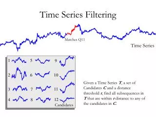
Time Series Filtering Matches Q11 Time Series 1 5 9 Given a Time Series T, a set of Candidates Cand a distance threshold r, find all subsequences in T that are within r distance to any of the candidates in C. 2 6 10 11 3 7 12 4 8 Candidates
Filtering vs. Querying Query (template) Database Database Matches Q11 Best match 1 5 9 6 1 7 2 6 10 2 8 3 11 3 7 9 4 12 4 8 10 5 Database Queries
C 0 10 20 30 40 50 60 70 80 90 100 Q Euclidean Distance Metric Given two time series Q = q1…qn and C = c1…cn , the Euclidean distance between them is defined as:
C Q calculation abandoned at this point 0 10 20 30 40 50 60 70 80 90 100 Early Abandon During the computation, if current sum of the squared differences between each pair of corresponding data points exceeds r 2, we can safely stop the calculation.
Classic Approach Time Series 1 5 9 2 6 10 Individually compare each candidate sequence to the query using the early abandoning algorithm. 11 3 7 12 4 8 Candidates
U U L W L W Q Wedge Having candidate sequences C1, .. , Ck , we can form two new sequences U and L : Ui = max(C1i , .. , Cki ) Li = min(C1i , .. , Cki ) They form the smallest possible bounding envelope that encloses sequences C1, .. ,Ck . We call the combination of U and L a wedge, and denote a wedge as W. W = {U, L} A lower bounding measure between an arbitrary query Q and the entire set of candidate sequences contained in a wedge W: C1 C2
C1 (or W1 ) C2 (or W2 ) C3 (or W3 ) W(1, 2) Generalized Wedge • Use W(1,2) to denote that a wedge is built from sequences C1 and C2 . • Wedges can be hierarchally nested. For example, W((1,2),3) consists of W(1,2) and C3 . W((1, 2), 3)
Wedge Based Approach Time Series 1 5 9 • Compare the query to the wedge using LB_Keogh • If the LB_Keogh function early abandons, we are done • Otherwise individually compare each candidate sequences to the query using the early abandoning algorithm 2 6 10 11 3 7 12 4 8 Candidates
W(1,2) W((1,2),3) Q Q C1 (or W1 ) C2 (or W2 ) C3 (or W3 ) C1 (or W1 ) C2 (or W2 ) W(1, 2) W(1, 2) Examples of Wedge Merging W((1, 2), 3)
W3 W3 W3 W2 W(2,5) W(2,5) W5 C3 (or W3) W1 W1 W(1,4) W4 W4 C5 (or W5) W((2,5),3) W(((2,5),3), (1,4)) C2 (or W2) C4 (or W4) W(1,4) C1 (or W1) K = 5 K = 4 K = 3 K = 2 K = 1 Hierarchal Clustering Which wedge set to choose ?
Which Wedge Set to Choose ? • Test all k wedge sets on a representative sample of data • Choose the wedge set which performs the best
C1 (or W1 ) C2 (or W2 ) C3 (or W3 ) W(1, 2) Upper Bound on Wedge Based Approach • Wedge based approach seems to be efficient when comparing a set of time series to a large batch dataset. • But, what about streaming time series ? • Streaming algorithms are limited by their worst case. • Being efficient on average does not help. • Worst case Subsequence W((1, 2), 3)
W3 W3 W3 Subsequence W2 W(2,5) W(2,5) W((2,5),3) W5 W1 W1 W((2,5),3) W(1,4) W4 W4 W(((2,5),3), (1,4)) W(1,4) K = 5 K = 4 K = 3 K = 2 K = 1 W(1,4) If dist(W((2,5),3), W(1,4)) >= 2 r Triangular Inequality < r >= 2r ? fails cannot fail on both wedges
Experimental Setup • Datasets • ECG Dataset • Stock Dataset • Audio Dataset • We measure the number of computational steps used by the following methods: • Brute force • Brute force with early abandoning (classic) • Our approach (Atomic Wedgie) • Our approach with random wedge set (AWR)
ECG Dataset • Batch time series • 650,000 data points (half an hour’s ECG signals) • Candidate set • 200 time series of length 40 • 4 types of patterns • left bundle branch block beat • right bundle branch block beat • atrial premature beat • ventricular escape beat • r = 0.5 • Upper Bound: 2,120 (8,000 for brute force)
Stock Dataset • Batch time series • 2,119,415 data points • Candidate set • 337 time series with length 128 • 3 types of patterns • head and shoulders • reverse head and shoulders • cup and handle • r = 4.3 • Upper Bound: 18,048 (43,136 for brute force)
Audio Dataset • Batch time series • 37,583,512 data points (one hour’s sound) • Candidate set • 68 time series with length 51 • 3 species of harmful mosquitoes • Culex quinquefasciatus • Aedes aegypti • Culiseta spp • Sliding window: 11,025 (1 second) • Step: 5,512 (0.5 second) • r = 2 • Upper Bound: 2,929 (6,868 for brute force)
Conclusions • We introduce the problem of time series filtering. • Combining similar sequences into a wedge is a quite promising idea. • We have provided the upper bound of the cost of the algorithm to compute the fastest arrival rate we can guarantee to handle.
Questions? All datasets used in this talk can be found at http://www.cs.ucr.edu/~wli/ICDM05/