Download
1 / 44
440 likes | 610 Vues
Clustering of Streaming Time Series is Meaningless. presentation by Rafal Ladysz after the original paper by Eamonn Keogh Jessica Lin Wagner Truppel Computer Science & Engineering, University of California-Riverside. interesting and important topic.

E N D
Clustering ofStreaming Time SeriesisMeaningless presentation by Rafal Ladysz after the original paper by Eamonn Keogh Jessica Lin Wagner Truppel Computer Science & Engineering, University of California-Riverside
interesting and important topic • foreward of the original paper reads: • “Clustering is perhaps the most frequently used data mining algorithm, being useful in it's own right as an exploratory technique, and also as a subroutine in more complex data mining algorithms such as rule discovery, indexing, summarization, anomaly detection, and classification” • “Time series data is perhaps the most frequently encountered type of data examined by the data mining community” • thus, a lot of interest, works, papers, conferences on these two, nevertheless • “it has never appeared in the literature” what the title claims
QUIZ questions (asked upfront) • what are two main ways of clustering time series data? (name and describe each in one sentence) • one can “convert” hierarchical clustering into k-means clustering: which of these two is deterministic (if any)? • what method can help subclustering time series work?
time series (TS) mini-primer • intuitive definition: sequence of real numbers (usually acquired in equal time intervals) • examples of experimental time series • meteorological observations • EEG, EKG, patient’s temperature (medical) • laser light intensity measured • stock market indices • predator-prey population recorded • possible division • periodic/non-periodic • stochastic (random)/chaotic (deterministic)
possible TS hierarchy tree the leaf nodes refer to theactual representation, and the internal nodes refer to the classification of the approach credit: Keogh et al.
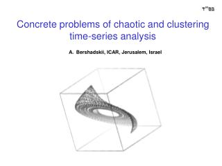
TS: illustration S&P laser Lorenz earthquake chaotic
mining TS • general examples • anomaly detection (deviation from some mean value, e.g. monitoring functioning of space shuttle) • classification/ forecasting • rule discovery (surprising/interesting patterns) • particular example (of my current interest) • detecting chaos in dynamic TS data streams • getting insight of the underlying system’s dynamics • computing some crucial parameter(s) • possible applications of the above • EEG • stock market • weather-related catastrophes (extremally complex)
TS – similarity issue • in many (though not all) cases similarity is necessary to investigate TS data • we need some measure of similarity to mine TS • classification, e.g. ECG patterns of new patients as indicator of heart deseases with known ECG pattern • clustering, e.g. groupping websites with similar traffic patterns • association, e.g. a plateau followed by a sudden decrease in EEG an epileptic seizure can happen • we need it for searching particular pattern (once we can use techniques/tools to mine TS)
TS similarity – possible measures • in general – there are many and what to use depends on the application • an obvious similarity measure is one based on Euclidean distance (with its pros and cons): • each sequence as a point in n-dimensional Euclidean space, where n = length of TS points then similarity Lp between TS sequences X, Y is Lp = (i=1n |xi – yi|p)1/p • old problem of dimensionality curse exists • thus scalability is desired and enforces • trade off between accuracy and efficiency
Euclidean distance for TS in action credit: A. K. Singh
similarity of TS – when we use it • Indexing problem • find all lakes whose water level fluctuations are similar to X • Subsequence Similarity problem • find out other days in which stock X had similar movements as today • Clustering problem • group regions that have similar sales patterns • Rule Discovery problem • find rules such as “if stock X goes up and Y remains the same, then Z will go down soon”
clustering algorithms: quick look at three of them • well known k-means • choosing k: the number of clusters to generate • initializing k centers of clusters to be generated • keep re-estimating k clusters’ centers • ... greedy • ... converges but not (necessarily) to global minimum • ... depends on initialization is step 2 • stops when no changes (in cluster membership) • hierarchical clustering • density-based clustering
hierarchical clustering: step by step 1. distances between objects: compute and put into distance matrix 2. search through distance matrix to find two closest (i.e. most similar) objects (clusters in next iterations) 3. join the two to get cluster of at least two objects 4. update distance matrix (new clusters generated) 5. repeatstep 2 until there is one cluster of all objects (from step 1) Q: is it bottom up (aglomerative) or top down?
hierarchical clustering: illustration averages • TS being clustered hierarchically - starting with 10 sequences • sliding either way along green line the “cut off” line determines • k (clusters) - thus determines “bottom-up” or “top-down” way • so we can “convert” hierarchical clustering to k-means cluster.
hierarchical clustering summary • it produces the same results every time with a given set of data (unlike k-means clustering) • cons: • splitting or merging “irreversible” in next iterations (i.e. no element redistribution among clusters) • poor scaling (quadratic in input size) • pros: • no input parameters (like number of clasters k) • simplicity • can be integrated with other clustering methods
density-based clustering (DBC) based on density - local cluster criterion recognizes clusters as “dense regions” major features: discover clusters of arbitrary shape handle noise one scan need density parameters as termination condition sources and algorithms: DBSCAN: Ester, et al. (KDD’96) OPTICS: Ankerst, et al (SIGMOD’99). DENCLUE: Hinneburg & D. Keim (KDD’98) CLIQUE: Agrawal, et al. (SIGMOD’98)
TS and its subsequences • formally, TS can be expressed as an ordered set of m variables or a point inm-dim space TS = t1, t2, ..., tm • this formality enables applying clustering to a set of TS sequences as if they were such points • Cp denotes a subsequence of length w of a TS, where w < m: Cp = tp, tp+1, ..., tp+w-1, 1 p m-w+1 • a technique of “sliding window” (of size w) is a useful concept here
subsequences via sliding window • sliding window extracts all subsequences Cp described earlier from a given TS • a matrix S of all such subsequences can be built by moving the sliding window across a given TS • and placing subsequence Cp in the pth row of S whose size is (m-w+1) times w far left: first eight subsequences Cp, each of length 16; middle: C67 of the same length
sliding window and its matrix • denoting all possible subclusters Cp C1 = {t1, t2, …, t10} C2 = {t2, t3, …, t11} Cm-w = {tm-9, tm-8, …tm} • and their corresponding matrix S:
meaninglessness of STS clustering • to demonstrate meaninglessness of STS clustering two algorithms have been used: • k-means • hierarchical clustering • important remark: to minimize any “methodological” bias, the whole clustering (besides STS sliding window clustering) has been performed to provide control results for comparison
variability of k-means: one data set • let A, B denote cluster centers derived from two different runs of k-means algorithm over the same data set (expect different results): • the cluster_distance(A, B) defines the distance between two sets of clusters: A and B remark: the above definition enforces closest pairs from A, B
variability of k-means: two data sets • applying this approach for different data sets • experiment: performing 3 random restarts of k-means (applying sliding window) on a stock market dataset • set X: the 3 resulting sets of cluster centers • similarly with 3 random runs of k-means on a random walk dataset • set Y: the resulting cluster centers
more definitions • denote the avaragecluster_distance between each set of cluster centers in Xto each other set of cluster centers in X (as it was for one data set) by within_set_X_distance • denote the average cluster distance between each set of cluster centers in Xto cluster centers in Y by between_set_X_and_Y_distance
a brief analysis of the claster meaningfullness(X, Y) • numerator (within set distance X) measuring clustering algorithm’s sensitivity to initial conditions (seeds); briefly: it asumes zero for same results • on the other hand: there is no reason for similarity of clustering results for two different (and unrelated) data sets: briefly: denominator (between set X and Y distance) should be (relatively) large • overall tendency: claster meaningfullness(X, Y) 0 if X, Y differ
experiment: STS vs whole clustering • to obtain control set of results (for comparison) • the same experiment has been repeated by k-means • for the same data • using whole clustering method (i.e. randomly extracted subsequences) • entire process has ben repeated 100 times for every combination of parameters k and w: k={3, 5, 7, 11} w={8, 16, 32} • results: first surprise!!! comparison: whole (yellow) vs. STS Z-axis: meaningfulness value
same experiment: hierarchical clust. • having proven meaningless of k-means clustering of STS, • the experiment has been performed using hierarchical clustering • new challenge: defining distance between two clusters: • linkage method - applicable for bottom-up clustering cluster objects can be based on different methods: Single Linkage: the minimum distance between them (nearest neighbour rule) Complete Linkage: the maximum distance between them (furthest neighbour rule) Average Linkage: the average distance between all pairs of objects (one member of the pair must be from a different cluster) cluster meaningfullness comparison: whole clustering vs. STS clustering using hierarchical approach; data used: S&P 500; again,no significant difference!
why it is really surprising: dissimilarity of data sets • the below two TS are very dissimilar • neverteless, the experimental results obtained for buoy sensor and ocean TS (using k-means) continue showing meaningless of STS clust.
preliminary conclusions • the authors reported similar results • using other clustering algorithms, e.g. EM, SOMs (self-organizing featire maps) • applied to more than 40 data sets • using Euclidean, L, Mahalanobis and “time warping distances” • and normalization techniques • and for all of those combinations observed • whole clustering of TS usually is to be meaningful • sliding windowclustering of STS never is meaningful
looking for explanation • another comparison of both methods • using cylinder, bell and funnel data sets • 30 instances generated for each pattern (90 total) • k-means applied (k = 3) • all (three) clusters have been recognized • close resemblance found
more results, more surprises • the 90 TS data sets (generated) have been concatenated to one long TS • sliding window: w =128, k-mean with k = 3 (as expected!) • the above graph illustrates obtained result, i.e. cluster centers found by subsequence clustering (using sliding the window described above) • a big surprise: the lines are sinusoids – no resemblenceto any patterns in data sets used as it was for whole clustering • summarizing: regardless clustering algorithm, number of clusters, datasets used: if w << m and STS then sinusoid
summarizing once again • the authors conclude: • obtained approximate sinusoids with STS clusteringregardless of the clustering algorithm, the number of clusters, or the dataset used • if sinusoids appear as cluster centers for every dataset, then clearly it will be impossible to distinguishone dataset’s clusters from another • this is all the more true as the “joint phase” of the sinusoids is arbitrary – does not depend on any input-related parameters • recall that independence on such parameters was defined as mininglessness
another concept: Hidden Constraint • let’s agree with the following theorem: for any TS dataset, if TS is clustered using sliding windows with w<<m, then the mean ofall the data (i.e. case for k=1) will be approximately constant (I’m not sure why they use the tem “vector” here) space shuttle flutter speech power data koski ecg rarthquake chaotic cylinder random walk balloon “visual proof” of the theorem w = 32, k = 1, 10 dissimilar datasets right: resulting cluster centers (no rescaling has been done)
(more) intuitive proof of the theorem • consider a time series TS and a single datapoint ti, where w i m-w+1 • as the sliding window pass by, ti goes on to appear exactly once in every possible location within it • ti contribution to the overall shape is the same every where and must be a horizontal line • the average of many horizontal lines is just another horizontal line ti
trivial match: the main idea • consider TS subsequence Cp being a member of a cluster • searchng for similar subsequences, where one can expect them to be? • in closest proximity! thus: ..., Cp-2,Cp-1,Cp+1,Cp+2, ...
trivial match: definition • trivial match: C and M are subsequences beginning at p and q, respectively, while R is a distance • M is a trivial matchto C of order R: if eitherp = q orthere does not exist a subsequence M’ beginning at q’ and such that D(C, M’) > R, and eitherq < q’ < p orp < q’ < q C M’ M p=q p<q’<q
trivial match: observation • smooth, slowly changing subsequences tend to have many trivial matches • rapidly changing subsequences (i.e. their features) tend to have very few trivial matches • the smooth pattern is surrounded by many trivial matches – sort of “compelling” as a cluster center • highly featured, noisy pattern has few trivial matches, often ignored as a cluster center candidate illustration of the observation A: TS sequence with a cluster of 3 square waves; w = 64 B: number of trivial matches
tentative conclusions • smooth patterns are surrounded by many trivial matches • extremely promising cluster center in clustering algorithms • D(C,M) < R • in 1920’s, Evgeny Slutsky demonstrated that any noisy time series will converge to a sine wave after repeated applications of moving window smoothing • STS, though not exactly such, is closely related
sine qua non for STS cluster • the weighted mean of the k patterns must sum to a horizontal line (constant line) • rach of the k patterns must have approximately equal number of trivial matches • the chances of both conditions being met is essentially zero…
a “tentative” solution • proposed a method as an existence proof only that such an algorithm exists at all (conceptually) • presented below is a motif-based clustering • definition of K-motifs: • given TS, a subsequence of length n, distance range R • the most significant motif in TS called 1-Motif is the subsequence C1 with the highest count of non-trivial matches • each subsequent K-motif in TS is the CK which differs from C1 in that additionaly: D(CK, Ci) > 2R for all 1 i < K the motif (red) occurs 4 times; winding(4) dataset used
motif vs. cluster • when mining motifs, we must specify an additional parameter R • assuming the distance R is defined as Euclidean, motifs always define circular regions in space, whereas clusters may have arbitrary shapes • motifs generally define a small subset of the data, and not the entire dataset • the definition of motifs explicitly eliminates trivial matches
algorithm for motif-based clustering • decide on a value for k • discover the K-motifs in the data, for K=kc (c is some constant about 2 to 30) • run k-means, or k partitional hierarchical clustering, or any other clustering algorithm on the subsequences covered by K-motifs
experimental results • repeated experiment for searching cluster centers for cyllinder-bell-funnel trio • the results obtained are “okey”, i.e. they resemble the original patterns (see right) of the three TS data sets (as well as results obtained using whole clustering approach)
side remark: another point of view • by Anne Denton • needlessly to say her Ph.D. thesis was entitled “Fast kernel-density-based classification and clustering using P-trees”, a good motivation to defend meaningfullness of STS • experimental setup: • data sets “halved” before clustering • comparing derived cluster centers from both halves using meaningfullness measure (“within/between”) and similar cluster distance measure • claim: such a test is “stricter” than that reported so far (based on separate runs of k-means on same data) • conclusion: kernel-based clustering shows meaningful results for subsequence clustering
references • Keogh, Lin, Truppel: “Clustering of Time Series Subsequences is Meaningless: Implications for Previous and Future Research” • Han, Kamber: “Data mining. Concepts and Techniques” • Lin, Keogh, Lonardim Chiu: “A symbolic representation of Time Series...” • Denton: “Density-based Clustering of Time Series Subsequences” • Sprott: “Chaos and Time-Series Analysis” references of the above ones and many pertaining web pages THANK YOU!