Concrete problems of chaotic and clustering time-series analysis
320 likes | 584 Vues
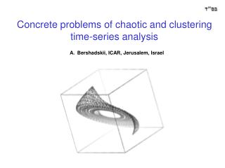
Bershadskii, ICAR, Jerusalem, Israel. Concrete problems of chaotic and clustering time-series analysis. Part I :. CHAOTIC TIME-SERIES ANALYSIS 1. Spectral discrimination between chaotic and stochastic (turbulent) time series 1.1 Exponential and power-law broad-band spectra

Concrete problems of chaotic and clustering time-series analysis
E N D
Presentation Transcript
Bershadskii, ICAR, Jerusalem, Israel Concrete problems of chaotic and clustering time-series analysis
Part I: • CHAOTIC TIME-SERIES ANALYSIS • 1. Spectral discrimination between chaotic and stochastic (turbulent) time series • 1.1 Exponential and power-law broad-band spectra • 1.2 Time-series related to low dimensional dynamic systems • 1.3 Time-series related to infinite dimensional dynamic system • 1.4 Singularities at complex times and the exponential spectra • 2. Hidden periods of chaotic time series • 2.1 Chaotic Sun • 2.2 Global temperature anomaly at millennial timescales • 2.3 Chaotic dynamics of atmospheric CO2and glaciation cycles • 2.4 Chaotic-chaotic climate response
STOCHASTIC DETERMINISTIC Scaling: no fixed scale Periodic: fixed scale (period) Chaotic: fixed scale Te
Rössler attractor • O.E. Rössler formulated a very simple continuous dynamical system generating chaotic solutions. • dx/dt = -(y + z) • dy/dt = x + a y • dz/dt = b + x z - c z • where a, b and c are parameters • ----------------------------------------------------- • Rössler, O. E. An equation for continuous chaos. Phys. Lett. A 35, 397 (1976). standard valuesa=0.15, b=0.20, c=10.0
Mackey-Glass delay differential equations A generic property, first observed by J.D. Farmer (1982) 0.00 0.04 0.08 0.10 t f B. Mensour and A. Longtin, Power spectra and dynamical invariants for delay-differential and difference equations, Physica D, 113, 1 (1998) =200, a=0.2, b=0.1
Nature of the exponential decay of the power spectra of the chaotic systems is still an unsolved mathematical problem. A progress in solution of this problem has been achieved by the use of the analytical continuation of the equations in the complex domain: U. Frisch and R. Morf, Intermittency in non-linear dynamics and singularities at complex times, Phys. Rev. 23, 2673 (1981). In this approach the exponential decay of chaotic spectrum is related to a singularity in the plane of complex time, which lies nearest to the real axis. Distance between this singularity and the real axis determines the rate of the exponential decay. For many interesting cases chaotic solutions are analytic in a finite strip around the real time axis. This takes place, in particular, for attractors bounded in the real domain (the Lorentz attractor, for instance). In this case the radius of convergence of the Taylor series is also bounded (uniformly) at any real time.
Singularities at complex times and the exponential spectra T/2 Fourier transform -T/2 The theorem of residues: the sum runs over all poles located in the relevant half plane,Rjbeing their residue and xj+ iyjtheir location. Asymptotic behavior of E(w) at large w yminis the imaginary part of the location of the pole which lies nearest to the real axis.
A delay chaotic system ? The 176y period is the third doubling of the period 22y. The 22y period corresponds to the Sun’s magnetic poles polarity switching. • Bershadskii, Europhys. Lett., 85, 49002 (2009).
If parameters of the dynamical system fluctuate periodically around their mean values with period Te, then the restriction of the Taylor series convergence (at certain conditions) is determined by Te, and the width of the analytic strip around real time axis equals Te/2p Parametric modulation with periodTe
arXiv:0903.2795 Chaotic climate response to periodic forcing A quasi-linear response to a weak periodic forcing High frequency tail of the spectrum of a reconstruction of Northern Hemisphere temperature anomaly for the past 2,000 years
Problem of glacial cycles 41 kyr 26 kyr 100 kyr ? The inclination of the Earth's orbit has a 100,000 year cycle relative to the invariable plane (the invariable plane is the plane that represents the angular momentum of the solar system).
The multi-millennium timescale changes in orientation change the amount of solar radiation reaching the Earth in different latitudes. In high latitudes the annual mean insolation (incident solar radiation) decreases with axial tilt, while it increases in lower latitudes. Axial tilt forcing effect is maximum at the poles and comparatively small in the tropics.
100,000-year problem of glacial cycles Observations show that glacial changes from -1.5 to -2.5 Myr (early Pleistocene) were dominated by 41 kyr cycle, whereas the period from -0.8 Myr to present (late Pleistocene) is characterized by approximately 100 kyr glacial cycles. While the 41 kyr cycle of early Pleistocene glaciation is readily related to the 41 kyr period of Earth’s axial tilt oscillations the 100 kyr period of the glacial cycles in last 0.8 Myr presents a serious problem. It was speculated in literature that influence of the axial tilt variations on global climate started amplifying around - 2.5 Myr, and became nonlinear from -0.8 Myr to present. Long term decrease in atmospheric CO2, which could result in a change in the internal response of the global carbon cycle to the axial tilt oscillations forcing, has been mentioned as one of the principal reasons for this phenomenon.
100,000-year problem of the glacial cycles A reconstruction of atmospheric CO2 based on deep sea proxies, for the past 650kyr. The data were taken fromW.H. Berger, Database for reconstruction of atmospheric CO2, IGBP PAGES/World Data Center-A for Paleoclimatology Data Contribution Series # 96-031. NOAA/NGDC Paleoclimatology Program, Boulder CO, USA
Chaotic response to strong periodic forcing by axial tilt Earth’s orbit variations with about 100 kyr period A quasi-linear response to aweakperiodic forcing Te = 1/fe = 41,000 yr Spectrum of the atmospheric CO2 fluctuations arXiv:0903.2795 Thus, the axial tilt oscillations period of 41 kyr is still a dominating factor in the chaotic CO2 fluctuations, although it is hidden for linear interpretation of the power spectrum
arXiv:0903.2795 Chaotic-chaotic climate response SSN Temperature Spectrum of temperature fluctuation in the semi-logarithmical scales (the reconstructed data for the last 10000 years – the interglacial warm period). Data at ftp://ftp.ncdc.noaa.gov/pub/data/paleo/ icecore/antarctica/epica_domec/edc3deuttemp2007.txt
PART II • CLUSTER ANALYSIS of TURBULENT (STOCHASTIC) TIME-SERIES • Telegraph approximation of turbulent signals • 2. Clustering and scaling: cluster-exponent • 3. Clustering and intermittency • 4. Clustering and spectral simulations: • Gaussian stochastic signal • 5. Isotherms clustering in cosmic microwave background and primordial turbulence
To neglect the amplitude fluctuations - to take into account the zero-crossing points only Scaling spectra b=1+2hg=1+h If we know scaling exponent for the telegraph approximation we know scaling exponent for the fullsignal! How much statistical information can be extracted from the zero-crossing points?
.. Let us suppose for simplicity that the velocity is a monofractal with Holder exponent h. Then, the fractal dimension of the zero-crossing set Z on the line is Hence, Where is variation of on scale . On the other hand,
K.R. Sreenivasan and A. Bershadskii, J. Stat. Phys., 125, 1141 (2006).
nt is running density of the • zero-crossing points with lag t Turbulent dissipation DISSIPATION EXPONENT
K.R. Sreenivasan and A. Bershadskii, J. Stat. Phys., 125, 1141 (2006).
Bershadskii, Phys. Lett., A360, 210 (2006) Spectral (Gaussian) simulation We use spectral simulation to illustrate that energy spectrum uniquely determines cluster-exponent for Gaussian-like turbulent signals. In these simulations we generate Gaussian stochastic signal with energy spectrum given as data (the spectral data are taken from the original velocity signals).
K.R. Sreenivasan and A. Bershadskii, J. Fluid Mech., 54, 477 (2006).
Cluster–exponent versus dissipation exponent K.R. Sreenivasan and A. Bershadskii, J. Stat. Phys., 125, 1141 (2006). If we know cluster-exponent we know dissipation exponent for the fullsignal! Zero-crossing points know all about scaling in turbulent signals
Bershadskii, Phys. Lett., A360, 210 (2006) Scaling: The motion of the scatterers in the last scattering surface imprints a temperature fluctuation, DT , on the CMB through the Doppler effect: wheren is the direction (the unit vector) on the sky, vb is the velocity field of the baryons evaluated along the line of sight, x = Ln, and gis the so-called visibility. where the metric scale r is replaced by number of the pixels, s, characterizing the size of the summation set (the random walk trajectory length). An analogy of the turbulent energy dissipation measure Cluster analysis:
Bershadskii, Phys. Lett., A360, 210 (2006) Standard deviation of the running density fluctuations against s for the CMB fluctuations in the 3 year WMAP
Reynolds number of the primordial turbulence • Bershadskii, Phys. Lett., A360, 210 (2006)