Download
1 / 24
240 likes | 255 Vues
Explore agricultural industries in Washington counties using input-output analysis. Compare crop and livestock data across counties using NAICS and SIC codes. Learn the benefits and drawbacks of NAICS. Implement the analysis in the R programming language for accurate results.

E N D
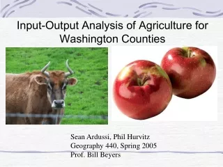
Input-Output Analysis of Agriculture for Washington Counties Sean Ardussi, Phil Hurvitz Geography 440, Spring 2005 Prof. Bill Beyers
Overview • Input-output analysis for each county in Washington State • Focusing on agricultural industries • Crops • Livestock
Data Sources • NAICS: employment, output, labor income • BEA (does not match official WAIO model) • USDA Census of Agriculture • WA Employment Security Department
NAICS – North American Industry Classification System (1997 +) SIC – Standard Industrial Classification (1997 and prior) SIC →NAICS
NAICS Benefits • Businesses that use similar production processes are grouped together • Expanded sectors to reflect changes in economy • Information sector • Service sector • NAFTA compatibility • USA, Canada, Mexico
NAICS Drawbacks • Less than 50% of SIC codes can be directly linked to a NAICS counterpart • Conversion from SIC to NAICS is subject to error of judgment
Methods • Washington State Input-Output Model (official WA Office of Financial Management model) • Implemented within an R statistical/programming language environment
R • Software for handling statistical operations • Good for dealing with tabular data • Handles generic and matrix math • Reads & writes standard files • Programming interface allows batch jobs
Example of R code # run the conflation and add to the employment matrix for (county in county.names) { # print (county) cty <- conflate.esd(county, 19) employment <- cbind(employment, cty) } colnames(employment) <- county.names # sum across rows to get WA totals of employment wa.employment <- rowSums(employment) wa.employment.sum <- sum(wa.employment) # make location quotients LQs <- NULL LQs.modified <- NULL for (i in 1:ncol(employment)) { lqs.county <- NULL lqs.county.modified <- NULL county.sum <- sum(employment[,i]) for (j in 1:nrow(employment)) { lq.local.component <- employment[j, i] / county.sum lq.state.component <- wa.employment[j] / wa.employment.sum lq <- lq.local.component / lq.state.component ifelse (lq < 1, lq.mod <- lq, lq.mod <- 1) lqs.county <- c(lqs.county, lq) lqs.county.modified <- c(lqs.county.modified, lq.mod) } LQs <- cbind(LQs, lqs.county) LQs.modified <- cbind(LQs.modified, lqs.county.modified) }
Results • Comparison of metrics across counties • Location quotients • Output • Employment • Labor income
Location Quotients: Livestock Livestock • High Counties • Adams – 11.82 • Pacific – 8.62 • Mason – 8.11 • Yakima – 6.86
Location Quotients: Livestock Livestock • Low Counties • King – 0.13 • Spokane – 0.16 • Pierce – 0.62 • Snohomish – 0.82
Location Quotients: Crops Livestock • High Counties • Okanagon – 17.11 • Douglas – 15.8 • Klickitat – 12.24 • Grant – 10.82
Location Quotients: Crops Livestock • Low Counties • King – .03 • Kitsap – .064 • Spokane – .089 • Snohomish – .114
Limitations • Needed to conflate data sets • Needed to impute data • Excel format not easy to translate to R
Benefits • R code can be altered and simply run again to generate output statistics & figures • Reduces user error when programmed correctly
Conclusions • Different counties in the State vary widely with respect to agricultural economics • Increased urbanization will have different effects on different locations in the State