Download
1 / 7
70 likes | 280 Vues
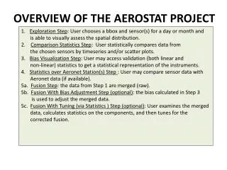
OVERVIEW OF THE AEROSTAT PROJECT. Exploration Step : User chooses a bbox and sensor(s) for a day or month and is able to visually assess the spatial distribution. 2. Comparison Statistics Step : User statistically compares data from

E N D
OVERVIEW OF THE AEROSTAT PROJECT • Exploration Step: User chooses a bbox and sensor(s) for a day or month and • is able to visually assess the spatial distribution. • 2. Comparison Statistics Step: User statistically compares data from • the chosen sensors by timeseries and/or scatter plots. • Bias Visualization Step: User may access validation (both linear and • non-linear) statistics to get a statistical representation of the instruments. • Statistics over Aeronet Station(s) Step : User may compare sensor data with • Aeronet data (if available). • 5a. Fusion Step: the data from Step 1 are merged (raw). • 5b. Fusion With Bias Adjustment Step (optional): the bias calculated in Step 3 • is used to adjust the merged data. • 5c. Fusion With Tuning (via Statistics ) Step (optional): User examines the merged • data, calculates statistics on the components, and then tunes for the • corrected fusion.
1. Exploration Step: User clicks on bbox for a select day (or month) and then chooses sensor(s). Ex. MODIS Terra & Aqua, OMI, MISR, and MODIS Aqua Deep Blue. This gives the user a glance at the data and a way to visually assess the spatial distribution(s) for each individual sensor for that day (or month). Data Source: L2 Database
User statistically compares data from the the chosen sensors via timeseries and/or scatter plots. 2. Comparison Statistics Step: MODIS Aqua OMI MODIS Aqua MODIS Aqua Computed on the fly? MISR MODIS Terra
User may access validation (both linear and non-linear) statistics to get a statistical representation of the instruments. 3. Bias Visualization Step: User can filter by region and season. MODIS Aqua Other filters, such as surface type and clouds, may be utilized, as well. A bias might then be inferred and “stored” in a Bias Adjustment “database” MODIS Terra Data Source: validation database PDF
4. Statistics over Aeronet Station(s) Step: If an Aeronet station is available, the user may wish to compare sensor data with Aeronet data via timeseries overlay or scatter plot. Aeronet MOD (this plot doesn’t depict actual data) Data Source: MAPSS database
5a. Fusion Step: The data from Step 1 are merged. 5b. Fusion With Bias Adjustment Step (optional): + PDF Data Source: Bias Adjustment “database” (calculated in Step 3)
5c. Fusion With Tuning (via Statistics) Step (optional): User examines the merged data, calculates statistics on the components, and then tunes for the corrected fusion. Statistics MODIS Terra + MODIS Aqua Fused Data Aeronet (if available) Time Note: If Aeronet data is not available, then the user will need to choose a sensor to act as a baseline to compute statistics.