Advanced Techniques in Parallel Imaging Reconstruction for Improved MRI Quality
Explore the world of parallel imaging reconstruction to reduce acquisition times, enhance resolution, and minimize artefacts in MRI scans. Understand k-space principles, coil sensitivities, and linear algebra techniques for efficient reconstruction. Learn about SENSE, GRAPPA, coil normalization, and handling difficult regions to optimize image quality.

Advanced Techniques in Parallel Imaging Reconstruction for Improved MRI Quality
E N D
Presentation Transcript
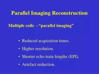
Parallel Imaging Reconstruction • Reduced acquisition times. • Higher resolution. • Shorter echo train lengths (EPI). • Artefact reduction. Multiple coils - “parallel imaging”
K-space from multiple coils coil views coil sensitivities multiple receiver coils k-space simultaneous or “parallel” acquisition
Undersampled k-space gives aliased images SAMPLED k-space k-space Fourier transform of undersampled k-space. coil 1 FOV/2 coil 2 Dk = 2/FOV Dk = 1/FOV
SENSE reconstruction ra p1 coil 1 rb coil 2 p2 Solve for ra and rb. Repeat for every pixel pair.
Image and k-space domains object coil sensitivity coil view Image Domain multiplication x = s c r FT k-space convolution = R C S coil k-space “footprint” object k-space
Generalized SMASH image domain product k-space convolution matrix multiplication = R S C gSMASH1 matrix solution 1Bydder et al. MRM 2002;47:16-170.
Composition of matrix S Acquired k-space coil 1 coil 2 hybrid-space data column S FTFE process column by column
Coil convolution matrix C C FTPE coil sensitivities hybrid space cyclic permutations of &
missing samples (can be irregular) gSMASH coil 1 = coil 2 S R C requires matrix inversion
Linear operations • Linear algebra. • Fourier transform also a linear operation. • gSMASH ~ SENSE • Original SMASH uses linear combinations of data.
SMASH - + - + + + + + PE weighted coil profiles sum of weighted profiles Idealised k-space of summed profiles 1st harmonic 0th harmonic
SMASH data summed with 0th harmonic weights = R data summed with 1st harmonic weights easy matrix inversion
GRAPPA • Linear combination; fit to a small amount of in-scan reference data. • Matrix viewpoint: • C has a diagonal band. • solve for R for each coil. • combine coil images.
Linear Algebra techniques available • Least squares sense solutions – robust against noise for overdetermined systems. • Noise regularization possible. • SVD truncation. • Weighted least squares. Absolute Coil Sensitivities not known.
Coil Sensitivities • All methods require information about coil spatial sensitivities. • pre-scan (SMASH, gSMASH, SENSE, …) • extracted from data (mSENSE, GRAPPA, …)
One-off extra scan. Large 3D FOV. Subsequent scans run at max speed-up. High SNR. Susceptibility or motion changes. No extra scans. Reference and image slice planes aligned. Lengthens every scan. Potential wrap problems in oblique scans. Merits of collecting sensitivity data Pre-scan In data
PPI reconstruction is weighted by coil normalisation coil data used (ratio of two images) reconstructed object • c load dependent, no absolute measure. • N root-sum-of-squares or body coil image.
Handling Difficult Regions body coil raw (array/body) array coil image thresholded raw local polynomial fit filtered threshold region grow www.mr.ethz.ch/sense/sense_method.html
ra p1 rb p2 SENSE in difficult regions coil 1 coil 2
Sources of Noise and Artefacts • Incorrect coil data due to: • holes in object (noise over noise). • distortion (susceptibility). • motion of coils relative to object. • manufacturer processing of data. • FOV too small in reference data. • Coils too similar in phase encode (speed-up) direction. • g-factor noise.
Tips • Reference data: • avoid aliasing (caution if based on oblique data). • use low resolution (jumps holes, broadens edges). • use high SNR, contrast can differ from main scan. • Number of coils in phase encode direction >> speed-up factor. • Coils should be spatially different. • (Don’t worry about regularisation?)