Reconstruction with Adaptive Feature-Specific Imaging
This paper discusses the innovative approach of Adaptive Feature-Specific Imaging (AFSI) for object reconstruction, detailing its advantages over traditional methods. Utilizing Principal Component Analysis (PCA) and Hadamard bases, AFSI enhances measurement signal-to-noise ratio (SNR), operational efficiency, and diminishes hardware complexity. The study presents frameworks for both sequential and parallel architectures, demonstrating significant reductions in reconstruction error (RMSE) through the adaptation of projection vectors. Findings highlight AFSI's superior performance with diverse training data, making it a groundbreaking methodology in optical imaging.

Reconstruction with Adaptive Feature-Specific Imaging
E N D
Presentation Transcript
Reconstruction with Adaptive Feature-Specific Imaging Jun Ke1 and Mark A. Neifeld1,2 1Department of Electrical and Computer Engineering, 2College of Optical Sciences University of Arizona Frontiers in Optics 2007
Outline • Motivation for FSI and adaptation. • Adaptive FSI using PCA/Hadamard features. • Adaptive FSI in noise. • Conclusion. Frontiers in Optics 2007
object reconstruction object Imaging optics light collection Reconstruction matrix G (NxM) feature single detector DMD projection vector FSI benefits: • Lower hardware complexity • Smaller equipment size/weight • Higher measurement SNR • High data acquisition rate • Lower operation bandwidth • Less power consumption LCD LCD G (NxM) LCD Motivation - FSI Reconstruction with Feature-specific Imaging (FSI) : Sequential architecture: Parallel architecture: Frontiers in Optics 2007
Adaptive PCA Static PCA Projection value Training samples for 2nd projection vector Projection axis 2 Testing sample Projection axis 1 Training samples Projection axis 1 Reconstruction Projection axis 2 Reconstruction Motivation - Adaptation • The design of projection vector effects reconstruction quality. • Using Principal Component Analysis (PCA) projection as example • Acquire feature measurements sequentially • Use acquired feature measurements and training data to adapt the next projection vector Frontiers in Optics 2007
Object estimate Object x Calculate R1from A1 Reconstruction Computational Optics Calculate f1 yi = fiTx Update Ai to Ai+1 according to yi Calculatefi+1 Ri+1 PCA-Based AFSI Adaptive FSI (AFSI) – PCA: K(1) nearest samples Projection axis 1 Selected samples K(1) nearest samples Projection axis According to 1st feature K(2) nearest samples Testing sample Projection axis 2 According to 2nd feature Testing sample i: adaptive step index Ai: ith training set K(i): # of samples for Ai+1 Ri: autocorrelation matrix of Ai fi: dominate eigenvector of Ai yi: feature value measured by fi • High diversity of training data helps adaptation Frontiers in Optics 2007
is the total # of features • Feature measurements: where, • Reconstructed object: • RMSE: PCA-Based AFSI Object examples (32x32): • Number of training objects: 100,000 • Number of testing objects: 60 Frontiers in Optics 2007
K(i) decreases iteration index i iteration index i Reconstruction from static FSI (i = 100) Reconstruction from AFSI (i = 100) PCA-Based AFSI AFSI – PCA: • RMSE reduces using more features • RMSE reduces using AFSI compare to static FSI • Improvement is larger for high diversity data • RMSE improvement is 33% and 16% for high and low diversity training data, when M = 250. Frontiers in Optics 2007
Hadamard-Based AFSI AFSI – Hadamard: • Projection vector’s implementation order is adapted. First 5 Hadamard basis ←Static FSI AFSI→ projection axis 1 projection axis 2 projection axis 1 sample mean <A1> Selected samples according to 1st feature K(2) nearest samples testing sample testing sample K(1) nearest samples K(1) nearest samples according to 2nd feature sample mean <A2> • Sample mean for training set Ai is <Ai> • yj= fiT<Ai>j = 1,…,M • max{yj} corresponds to the dominant Hadamard projection vector Frontiers in Optics 2007
Selected samples according to 1st 2 features <Ai> Object estimate K(1) nearest samples Sort Hadamard basis vectors Reconstruction Object x sample mean Choose f1~fL Computational Optics yiL+j = f iL+jTx (j=1,…,L) projection axis 2 testing sample Choose fiL+1 ~ f(i+1)L Update Ai to Ai+1 according to yiL+j projection axis 1 Sort <Ai+1> Hadamard-Based AFSI AFSI – Hadamard: • L : # of features in each adaptive step <Ai>: sample mean of Ai fi: ith Hadamard vector for Ai Frontiers in Optics 2007
L decreases L increases K(i) decreases number of features M = Li number of features M = Li Reconstruction from static FSI Hadamard-Based AFSI AFSI – Hadamard: • RMSE reduces in AFSI compared with static FSI • RMSE improvement is 32% and 18% for high and low diversity training data, when M = 500 and L = 10. • AFSI has smaller RMSE using small L when M is also small • AFSI has smaller RMSE using large L when M is also large Reconstruction from adaptive FSI Frontiers in Optics 2007
Object estimate <A1> Object x Sort Hadamard bases Reconstruction Computational Optics Calculate Ri for Ai yiL+j = fiL+jTx+niL+j (j = 1,2,…L) Choose f1~fL ChoosefiL+1~f(i+1)L from de-noising yiL+j Sort Update Ai to Ai+1 according to <Ai+1> Hadamard-Based AFSI – Noise AFSI – Hadamard: • T : integration time • σ02 = 1 • detector noise variance: σ22 = σ02/T • Hadmard projection is used because of its good reconstruction performance • Feature measurements are de-noised before used in adaptation • Wiener operator is used for object reconstruction • Auto-correlation matrix is updated in each adaptation step Frontiers in Optics 2007
High diversity training data; σ02 = 1 High diversity training data; σ02 = 1 AFSI – adapted Rx AFSI – fixed Rx L decreases L increases K(i) decreases Static FSI Hadamard-Based AFSI – Noise • RMSE in AFSI is smaller than in static FSI • RMSE is reduced further by modifyingRx in each adaptation step • RMSE improvement is larger using small L when M is also small • RMSE is small using large L when M is also large Frontiers in Optics 2007
High diversity training data; σ02 = 1 High diversity training data; σ02 = 1 Hadamard-Based AFSI – Noise T : integration time/per feature; M0: the number of features Total feature collection time = T × M0 Increasing T • Reducing Measurement error • Losing adaptation advantage Trade-off Minimum total feature collection time Frontiers in Optics 2007
Conclusion • Noise free measurements: • PCA-based and Hadmard-based AFSI system are presented • AFSI system presents lower RMSE than static FSI system • Noisy measurements: • Hadamard-based AFSI system in noise is presented • AFSI system presents smaller RMSE than static FSI system • There is a minimum total feature collection time to achieve a reconstruction quality requirement Frontiers in Optics 2007

