Download
1 / 26
260 likes | 321 Vues
Explore entropy rate balance in closed systems & control volumes, with in-depth examples and calculations for evaluating energy and entropy transfers. Understand the significance of entropy production and its impact on thermodynamic performance.

E N D
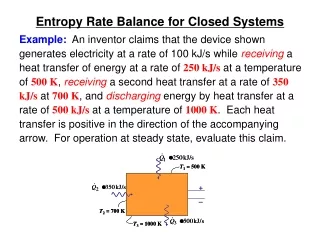
Entropy Rate Balance for Closed Systems Example: An inventor claims that the device shown generates electricity at a rate of 100 kJ/s while receiving a heat transfer of energy at a rate of 250 kJ/s at a temperature of 500 K, receiving a second heat transfer at a rate of 350 kJ/s at 700 K, and discharging energy by heat transfer at a rate of 500 kJ/s at a temperature of 1000 K. Each heat transfer is positive in the direction of the accompanying arrow. For operation at steady state, evaluate this claim.
∙ Since σ is negative, the claim is not in accord with the second law of thermodynamics and is therefore false. Entropy Rate Balance for Closed Systems 0 • Applying an energy rate balance at steady state Solving The claim is in accord with the first law of thermodynamics. 0 • Applying an entropy rate balance at steady state Solving
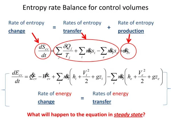
where and account, respectively, for rates of entropy transfer accompanying mass flow at inlets i and exits e. Entropy Rate Balance for Control Volumes • Like mass and energy, entropy can be transferred into or out of a control volume by streams of matter. • Since this is the principal difference between the closed system and control volume entropy rate balances, the control volume form can be obtained by modifying the closed system form to account for such entropy transfer. The result is (Eq. 6.34)
where1 and 2 denote the inlet and exit, respectively, and is the common mass flow rate at these locations. Entropy Rate Balance for Control Volumes • For control volumes at steady state, Eq. 6.34 reduces to give (Eq. 6.36) • For a one-inlet, one-exit control volume at steady state, Eq. 6.36 reduces to give (Eq. 6.37)
Entropy Rate Balance for Control Volumes Example: Water vapor enters a valve at 0.7 bar, 280oC and exits at 0.35 bar. (a) If the water vapor undergoes a throttling process, determine the rate of entropy production within the valve, in kJ/K per kg of water vapor flowing. (b) What is the source of entropy production in this case? (a) For a throttling process, there is no significant heat transfer. Thus, Eq. 6.37 reduces to 0 →
(8.6295 – 8.3162) kJ/kg∙K =0.3133 kJ/kg∙K Finally Entropy Rate Balance for Control Volumes Solving From Table A-4, h1 = 3035.0 kJ/kg, s1 = 8.3162 kJ/kg∙K. For a throttling process, h2 = h1 (Eq. 4.22). Interpolating in Table A-4 at 0.35 bar and h2 = 3035.0 kJ/kg, s2 = 8.6295 kJ/kg∙K. (b) Selecting from the list of irreversibilities provided in Sec. 5.3.1, the source of the entropy production here is the unrestrainedexpansion to a lower pressure undergone by the water vapor.
Entropy Rate Balance for Control Volumes Comment: The value of the entropy production for a single component such as the throttling valve considered here often does not have much significance by itself. The significance of the entropy production of any component is normally determined through comparison with the entropy production values of other components combined with that component to form an integrated system. Reducing irreversibilities of components with the highest entropy production rates may lead to improved thermodynamic performance of the integrated system.
Calculating Entropy Change • The property data provided in Tables A-2 through A-18, similar compilations for other substances, and numerous important relations among such properties are established using the TdS equations. When expressed on a unit mass basis, these equations are (Eq. 6.10a) (Eq. 6.10b)
(Eq. 6.10a) (Eq. 6.10b)
(Eq. 6.10a) (Eq. 6.10b) (Eq. 6.23)
Calculating Entropy Change • As an application, consider a change in phase from saturated liquid to saturated vapor at constant pressure. • Since pressure is constant, Eq. 6.10b reduces to give • Then, because temperature is also constant during the phase change (Eq. 6.12) This relationship is applied in property tables for tabulating (sg – sf) from known values of (hg – hf).
Calculating Entropy Change • For example, consider water vapor at 100oC (373.15 K). From Table A-2, (hg – hf) =2257.1 kJ/kg. Thus (sg – sf) = (2257.1 kJ/kg)/373.15 K = 6.049 kJ/kg∙K which agrees with the value from Table A-2, as expected. • Next, the TdS equations are applied to two additional cases: substances modeled as incompressible and gases modeled as ideal gases.
(Eq. 6.13) Calculating Entropy Change of an Incompressible Substance • The incompressible substance model assumes the specific volume is constant and specific internal energy depends solely on temperature: u = u(T). Thus, du = c(T)dT, where c denotes specific heat. • With these relations, Eq. 6.10a reduces to give • On integration, the change in specific entropy is • When the specific heat is constant
Calculating Entropy Change of an Ideal Gas • The ideal gas model assumes pressure, specific volume and temperature are related by pv = RT. Also, specific internal energy and specific enthalpy each depend solely on temperature: u = u(T), h = h(T), giving du=cvdT and dh=cpdT, respectively. • Using these relations and integrating, the TdS equations give, respectively (Eq. 6.17) (Eq. 6.18)
Calculating Entropy Change of an Ideal Gas • Since these particular equations give entropy change on a unit of mass basis, the constant R is determined from • Since cv and cp are functions of temperature for ideal gases, such functional relations are required to perform the integration of the first term on the right of Eqs. 6.17 and 6.18. • For several gases modeled as ideal gases, including air, CO2, CO, O2, N2, and water vapor, the evaluation of entropy change can be reduced to aconvenient tabular approach using the variable so defined by (Eq. 6.19) whereT'is an arbitrary reference temperature.
For air, Tables A-22 and A-22E provide so in units of kJ/kg∙K and Btu/lb∙oR, respectively. For the other gases mentioned, Tables A-23 and A-23E provide in units of kJ/kmol∙K and Btu/lbmol∙oR, respectively. Calculating Entropy Change of an Ideal Gas • Using so, the integral term of Eq. 6.18 can be expressed as • Accordingly, Eq. 6.18 becomes (Eq. 6.20a) or on a per mole basis as (Eq. 6.20b)
Calculating Entropy Change of an Ideal Gas Example: Determine the change in specific entropy, in kJ/kg∙K, of air as an ideal gas undergoing a process from T1= 300 K, p1 = 1 bar to T2 = 1420 K, p2 = 5 bar. • From Table A-22, we get so1 = 1.70203 and so2 = 3.37901, each in kJ/kg∙K. Substituting into Eq. 6.20a Table A-22
Calculating Entropy Change of an Ideal Gas • Tables A-22 and A-22E provide additional data for air modeled as an ideal gas. These values, denoted by pr and vr, refer only to two states having the same specific entropy. This case has important applications, and is shown in the figure.
Calculating Entropy Change of an Ideal Gas • When s2 = s1, the following equation relates T1, T2, p1, and p2 (Eq. 6.41) (s1 = s2, air only) wherepr(T)is read from Table A-22 or A-22E, as appropriate. Table A-22
Calculating Entropy Change of an Ideal Gas • When s2 = s1, the following equation relates T1, T2, v1, and v2 (Eq. 6.42) (s1 = s2, air only) wherevr(T)is read from Table A-22 or A-22E, as appropriate. Table A-22
(Eq. 6.22) (Eq. 6.21) Entropy Change of an Ideal Gas Assuming Constant Specific Heats • When the specific heats cv and cp are assumed constant, Eqs. 6.17 and 6.18 reduce, respectively, to (Eq. 6.18) (Eq. 6.17) • These expressions have many applications. In particular, they can be applied to develop relations among T, p, and v at two states having the same specific entropy as shown in the figure.
Entropy Change of an Ideal GasAssuming Constant Specific Heats • Since s2 = s1, Eqs. 6.21 and 6.22 become • With the ideal gas relations wherekis the specific ratio • These equations can be solved, respectively, to give (Eq. 6.43) (Eq. 6.44) • Eliminating the temperature ratio gives (Eq. 6.45)
Calculating Entropy Change of an Ideal Gas Example: Air undergoes a process from T1= 620 K, p1 = 12 bar to a final state where s2 = s1, p2 = 1.4 bar. Employing the ideal gas model, determine the final temperature T2, in K. Solve using (a)pr data from Table A-22 and (b) a constant specific heat ratio k evaluated at 620 K from Table A-20: k = 1.374. Comment. (a) With Eq. 6.41 and pr(T1) = 18.36 from Table A-22 Interpolating in Table A-22, T2 = 339.7 K Table A-22
Calculating Entropy Change of an Ideal Gas (b) With Eq. 6.43 T2 = 345.5 K Comment: The approach of (a) accounts for variation of specific heat with temperature but the approach of (b) does not. With a k value more representative of the temperature interval, the value obtained in (b) using Eq. 6.43 would be in better agreement with that obtained in (a) with Eq. 6.41.
Isentropic Turbine Efficiency • For a turbine, the energy rate balance reduces to 1 2 • If the change in kinetic energy of flowing matter is negligible, ½(V12 – V22) drops out. • If the change in potential energy of flowing matter is negligible, g(z1 – z2) drops out. • If the heat transfer with surroundings is negligible, drops out. where the left side is work developed per unit of mass flowing.
Isentropic Turbine Efficiency • For a turbine, the entropy rate balance reduces to 1 2 • If the heat transfer with surroundings is negligible, drops out.