First-Time User Guide: Band Structure Lab
430 likes | 544 Vues
Learn how to calculate electronic band structures, bandgaps, and effective masses in various semiconductor geometries using the Band Structure Lab tool. Understand the assembly of device Hamiltonians and the self-consistent E(k) calculation procedure.

First-Time User Guide: Band Structure Lab
E N D
Presentation Transcript
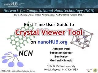
First-Time User Guide: Band Structure Lab Abhijeet Paul, Ben Haley, and Gerhard Klimeck NCN @Purdue University West Lafayette, IN 47906, USA
Table of Contents I • Introduction • Origin of bands (electrons in vacuum and in crystal) 5 • Energy bands, bandgap, and effective mass 6 • Different types of device geometries 7 • How is band structure calculated? 8 • Assembly of the device Hamiltonian 9 • Self-consistent E(k) calculation procedure 10 • Band Structure at a Glance 11 • Features of the Band Structure Lab 12 • A complete description of the inputs 14 • What Happens When You Just Hit Simulate? 20
Table of Contents II Some Default Simulations Circular silicon nanowire E(k) 23 Silicon ultra-thin-body (UTB) E(k) 25 Silicon nanowire self-consistent simulation27 Bulk Strain Sweep Simulation 29 Case Study 31 Suggested Exercises Using the Tool 34 Final Words about the Tool 35 References 36 Appendices 38 Appendix A: job submission policy for Band Structure Lab Appendix B: information about high symmetry points in a Brillouin zone Appendix C: explanation for different job types used in the tool
Origin of Bands: Electrons in Vacuum Schrödinger Equation Eigen Energy E(k) relationship E = Bk2 E Free electron kinetic energy Hamiltonian Continuous energy band Plane Waves (Eigen vectors) φ(k) = Aexp(-ikr) k • Single electron (in vacuum) Schrödinger Equation provides the solution: • Plane waves as eigen vectors • E(k) = Bk2 as eigen energy • Eigen energy can take continuous values for every value of k • E(k) relationship produces continuous energy bands k = Momentum vector E = Kinetic energy
Origin of Bands: Electrons in Crystal E(k) relationship Schrödinger equation Electron Hamiltonian in a periodic crystal E Discontinuous energy bands Periodic potential due to crystal (Vpp) GAP Atoms • An electron traveling in a crystal sees an extra crystal potential, Vpp. • Eigen vectors are no longer simple plane waves. • Eigen energies cannot take all the values. • Energy bands become discontinuous, thereby producing the BAND-GAPS. GAP GAP k
Energy Bands, Bandgap, and Effective Mass Energy bands Continuous bands Lattice constant = -π/a ≤ k ≤ π/a. This is called first BRILLOUIN ZONE. E(k) relation in this zone is called reduced E(k) relation E E E Bandgap E(k) relationship in periodic potential Vacuum electron E(k) relationship k k k Electron mass in vacuum = 9.1e-31kg Band Gap • Similar E(k) relationship • Now free electron mass is replaced by effective mass (m*) • Effective mass provides the energy band curvature π/a -π/a
Description of Geometries Nanowire 1D Periodic Bulk (3D periodic) Y Y X X • Nanowires have 3 cross-sectional shapes: circular, triangular, rectangular. • The semiconductor is represented atomistically for the E(k) calculation. • The oxide is treated as continuum material for self-consistent simulations. • X -> transport direction • Y,Z -> confinement directions Y Semiconductor X UTB (2D periodic) Oxide Z Z Z
How Band Structure is Calculated [4] Dispersion (E(k)) relation Y Bulk 3D periodicity X [2] Assemble device Hamiltonian [H] Z E E1 Band Gap Quantum well 2D periodicity E2 -π/a π/a E3 k In the Band Structure Lab, the device Hamiltonian is assembled using the semi-empirical tight-binding method. Device axis Quantum wire 1D periodicity [3] Diagonalized H provides eigen-energies [1] Select crystal dimensionality confinement periodicity
Assembly of the Device Hamiltonian Cation-Anion Coupling block [Vca] Anion-Cation Coupling block [Vac] Anion Onsite block [Hon_a] Cation Onsite block [Hon_c] Device Hamiltonian • Device Hamiltonian is assembled using semi-empirical tight-binding [TB] • Each atom is represented using • an onsite block [Hon_a or Hon_c]. • Coupling with nearest • neighbor is taken in coupling • blocks [Vac, Vca] • Size of these blocks depends on • the basis set and spin-orbit • coupling • Basis sets are made of • orthogonal atomic orbitals like • s,p,d,etc. • The Band Structure Lab uses • sp3d5s* basis set with 10 • basis functions Anion Cation
Self-consistent E(k) Calculation Procedure Electronic structure 20 band sp3d5s* model with spin orbit coupling • Appropriate for treating • atomic level disorder • Strain treatment at • atomic level • Structural, material & • potential variations • treated easily Zinc blend Top of the barrier ballistic transport Self consistent iteration scheme
Band Structure Lab at a Glance • What is the Band Structure Lab and what does it do?: • A C++ based code to perform electronic structure calculation • A tool powered by OMEN-BSLAB, C/C++ MPI based parallel code • Solves single electron Schrödinger equation in different types of semiconductor crystals using the semi-empirical tight-binding method: • For pure crystals with and without strain • For gates semiconductor systems with applied external biases for nanowires and ultra thin bodies (UTB) • Provides various information on an electron in a periodic potential • Energy bands • Effective masses and band-gaps This tool was developed at Purdue University and is part of the teaching tools on nanoHUB.org (AQME) .
Features of the Band Structure Lab • Calculation of energy dispersion(E(k)) for semiconductor materials: • In bulk (3D), Ultra Thin Bodies [UTB] (2D), and Nanowires (1D) • With and without strain in the system, it can handle: • Hydrostatic strain (equal strain in all directions) • Biaxial strain (equal strain on a plane) • Uniaxial strain (strain along any arbitrary axis) • Arbitrary strain (all directions have different strains) • Provides following information • Effective masses in bulk, nanowires, and UTBs • 3D dispersion for bulks in 1st Brillouin zone • Bandgaps and bandedges • Self-consistent simulations: • Provides charge and potential profile in nanowire FETs and in UTB DGMOS for the applied gate bias • Change in E(k) relation due to applied bias Screen shot from http://nanohub.org
Computational Aspects of Band Structure Lab • This tool has 3 levels of parallelism, namely: • Parallel over all the gate biases • Parallel over the kz point calculations for each Vg point • Parallel over the kx point calculation for each Kz point • Runs on multiple CPUs and on various clusters to provide a faster turn-around time for simulations • Tool has internal job submission method, depending on the kind of job the user wants to run • User can override these internal settings, but this should be done with care. See Appendix [A] for additional information on the job submission policy.
Inputs [1]: Device Structure Types of geometries and related parameters are selected on this page [2.3] Device Directions: [a] Transport direction (X) [100],[110],[111] [b] Confinement direction(Z) [c] 3rd orthogonal direction(Y) determined automatically [2] Device Information [1] Geometry [2.1] Job type: Bulk: Band structure calculation nanowire & UTB: [1] Band structure calculation [2] Band structure calculation under an applied bias [3] Material 4 Material Types: [a] Silicon [b] Gallium Arsenide [c] Indium Arsenide [d] Germanium 5 types of geometry [periodicity]: [1] Bulk [3D] [2] Circular nanowire [1D] [3] Rectangular nanowire [1D] [4] Triangular nanowire [1D] [5] Ultra thin body [2D] [2.2] Device Dimension: Depending on job type, select: [a] Dimension of NW or UTB semiconductor core in nm [b] Thickness of oxide in nm (This is available for self-consistent E(k) calculation.) Screen shot from http://nanohub.org
Inputs [2]: Electronic Structure Properties used to obtain the electronic dispersion are set on this page. [1] Tight Binding Model This is the basis, set model used for calculating the band structure. Presently, the sp3d5d* model is supported by the tool. • [2] Spin Orbit (SO) Coupling • This produces the effect of • electron spin on band structure. • Should be always “ON” for valence • bands. • Produces negligible effect on • conduction bands. • With SO on calculations are slower • due to larger matrix sizes. • [3] Dangling Bond Energy • This is the energy barrier set at the • external boundary of the structure. • This value is utilized to remove the • spurious states in the bandgap. Default • value of 30 eV is good. • Smaller value means lower barrier • and larger value means higher barrier. • Usually there is no need to change this value. Screen shot from http://nanohub.org
Inputs [3.a]: Analysis - Bulk This page provides options for the kind of simulations that can be run, depending on the selected geometry. Two types of simulations: bulk dispersion and strain sweep • Provide the initial and final % strain value • Provide number of points for strain sweep Strain sweep analysis: Effect of strain on E(k) Bulk dispersion [E(k)] calculation: Select the % strain value (eps_xx, eps_yy, eps_zz) along the 3 axes Explore bands [1] Along std. symmetry directions* [2] Along some symmetry directions* Strain Models [1] Bi-axial [2] Uniaxial [3] Hydrostatic [4] Arbitrary Only 3 models available for strain sweep analysis Show 3D E(k) Produces energy isosurface plots. User can set the kx, ky, kz region, as well as the energy limit. for the bands * See Appendix [B]
Inputs [3.b] Analysis - UTB Self-consistent calculation options E(k) calculation options Select Type of DGMOS N-type or P-type Depending on source-drain doping: Select Type of Band CB or VB Direction along which E(k) to be calculated* Select the number of sub-bands. • Bias selection: • Set gate bias. • Set drain bias. • Set gate work function. • Set semiconductor electron affinity. • Set device temperature. • Set DIBL. Select the number of k points. (Higher k points are good for a P-type simulation, but they increase the simulation time. Select the number of sub-bands. Select the number of k points. Select backgate configuration. Select the strain type and values. (Strain detail is the same as bulk) Set source/drain doping. Select the strain model. * See Appendix B
Inputs [3.c] Analysis - Wire Self-consistent calculation options E(k) calculation options Select Type of Gate all-around MOS N-type or P-type Depending on source-drain doping: Select Type of Band: CB or VB Select the number of sub-bands. Select the number of sub-bands. • Bias selection: • Set gate bias. • Set drain bias. • Set gate work function. • Set semiconductor electron affinity. • Set device temperature. • Set DIBL. Select number of k points. (Higher K points are good for a P-type simulation, but they increase the simulation time. Select the number of k points. Select the strain type and values. Strain detail is same as bulk. Set source/drain doping. Select strain model.
Inputs [4]: Advanced User Choice Allows the users to submit jobs on their cluster of choice See Appendix A for more details. Two clusters are available: NANOHUB (less CPUs) STEELE (larger CPUs) • Well suited for light* and • medium* job types • Has less delay in job submission • Self-consistent jobs should not be submitted as it may result it longer turn around time. • Well suited for medium* and • heavy* job types. • Has longer queue delays • during job submission. • Self-consistent jobs should • be submitted here. CAUTION:Do not change this option if you are not sure. The tool will automatically decide the simulation venue depending on the job type. * See Appendix A
What Happens When You Just Hit SIMULATE? [Bulk band structure]: Shows the all the energy bands. [Bulk central bands]: Shows only the conduction and 3 valence bands . [Bandgap/Bandedge information]: Provides information about band extrema and bandgap. [Effective mass information] : Provides conduction and valence band masses at high symmetry points. [Unitcell structure]: Shows 3D zinc-blend unitcell structure. [Atomic structure] : Shows a larger crystal of silicon. [Input decks]: Provides input decks used by OMEN-BSLAB. [Backend code log] : log of OMEN-BSLAB. [Timestamps] : Shows overall simulation time breakup. [Tool Run Log] : Shows the log of tool run. Default Outputs Default Inputs • Geometry -> Bulk • Material -> Silicon • TB Model ->sp3d5s* • Spin orbit -> on • Dangling bond energy: • 30eV • Bulk Ek simulation • Full Domain simulation • Strain -> none • Show 3D bands -> no • Advanced user choice -> • default. Screen shot from http://nanohub.org
What Happens When You Just Hit SIMULATE? (continued) [2] Central Bands [1] Bulk Bands Conduction Band Heavy hole Split-off hole [3] Band Info(Si) Light hole Valence Bands around Γ point [4] Silicon Unitcell Screen shots from http://nanohub.org
What Happens When You Just Hit SIMULATE? (continued) [5] Silicon effective masses Type of simulation Time stamps for overall simulation Conduction band masses Valence band masses [6] Timestamp and tool log Computational resource information Screen shots from http://nanohub.org
Default Circular Nanowire Simulation Inputs Outputs • Geometry -> circular nanowire • Material -> silicon • Wire diameter ->2.1nm • Transport direction(X) –>[100] • Confinement direction(Z) -> [010] • TB model ->sp3d5s* • Spin orbit -> on • Dangling bond energy -> 30 eV • CB and VB simulation • Number of bands ->10 • Number of k points -> 61 • Strain -> none • Advanced user choice -> no Conduction Bands [1] Wire Band Structure Valence Bands [2] Bandedge Information [3] Wire Unitcell Screen shots from http://nanohub.org
Default Circular Nanowire Simulation (continued) Outputs [6] Valence band transport eff. mass Job type [4] Longer Wire Structure Timestamps Resource utilization [5] Conduction band transport eff. mass [7] Simulation log Screen shots from http://nanohub.org
Default UTB Simulation Inputs Outputs • Geometry -> Ultra Thin Body (UTB) • Material -> silicon • Body thickness -> 1.0 nm • Transport direction(X) –>[100] • Confinement direction(Z) -> [010] • TB Model ->sp3d5s* • Spin orbit -> on • Dangling bond energy -> 30 eV • CB simulation • Full domain simulation • Number of bands ->10 • Number of k points -> 61 • Strain -> none • Advanced user choice -> no [1] CB E(k) Plots Γ->[100](X) Γ->[110](L) [2] Band Edge [3] Atomic structure Screen shots from http://nanohub.org
Default UTB Simulation (continued) Outputs [4] 2D Conduction Band [5] Simulation Log Job Type 2D CB no 1 Timestamps Resource utilization 2D CB no 2 Screen shots from http://nanohub.org
Nanowire Self-consistent Simulation Inputs Effect of gate bias on electronic structure Outputs • Geometry -> circular nanowire • Material -> silicon • Job type -> self-consistent E(k) • Wire diameter ->2.1 nm • Transport direction(X) –>[100] • Confinement direction(Z) -> [010] • TB Model ->sp3d5s* • Spin orbit -> off • Dangling bond energy -> 30 eV • N-type FET. • Number of bands ->10 • Number of k points -> 61 • Strain -> none • Vg = 0.2V, Vd = 0.05V, • Gate work function = 4.25 eV • Electron affinity = 4.05 eV • S/D doping = 1e20cm^-3. • Advanced user choice -> no • Comparison of initial and final Ek at • Vgs = 0.2 V • Due to the bias, the final Ek shifts lower to provide a charge. Screen shot from http://nanohub.org
Nanowire Self-consistent Simulation (continued) Outputs [2] 2D Charge profile [#/nm] Job-type [4] Source/Drain Fermi level [3] Ballistic current & injection velocity Timestamps Computational Resources [5] Output log Screen shots from http://nanohub.org
Bulk Strain Sweep Simulation Study the effect of biaxial strain on silicon bulk electronic structure Outputs Inputs • Geometry -> Bulk • Material -> Silicon • TB Model ->sp3d5s* • Spin orbit -> on • Dangling bond energy -> 30 eV • Strain sweep simulation • Strain -> Biaxial • Start strain value = -0.01 % • End strain value = 0.03 % • No. of strain points = 20. • Advanced user choice -> no [1] BandGap Variation [2] Band Edge Variation HH CB LH SO Screen shots from http://nanohub.org
Bulk Strain Sweep Silicon: Outputs [1] X valley electron eff. mass variation along different directions m_l(x) Electron masses do not vary much. • Other available plots • L valley electron eff. • mass variation • Light and split off • hole mass • variation • Variation in unitcell • structure • Output logs m111(x) m_t(x) m110(x) [1] Heavy Hole mass variation @ gamma valley hh111(Γ) Heavy hole masses do vary quite a bit. hh110(Γ) Screen shots from http://nanohub.org
Case Study: Nanowire Electronic Structure Study the effect of diameter variation on circular Silicon nanowire CB electronic dispersion Output plots Inputs • Geometry -> circular nanowire • Material -> silicon • Wire diameter ->[2.1,3.1,4.1,5.1,6.1] nm • Transport direction(X) –>[100] • Confinement direction(Z) -> [010] • TB model ->sp3d5s* • Spin orbit -> on • Dangling bond energy -> 30 eV • CB simulation • Number of bands ->10 • Number of k points -> 61 • Strain -> none • Advanced user choice -> no Band Edge vs wire diameter • CB bandedge goes higher in energy with a • decreasing diameter • As wire diameter increases, Ec value approaches bulk Ec value • All six silicon valleys lose degeneracy due to confinement
Case Study: Valley Splitting Output plots • Valley splitting has been • taken at gamma point. • In bulk the 6 CB lobes • are degenerate in • silicon, but split due to • confinement. • Valley splitting shows an • oscillatory behavior • which is expected since • the number of atomic • layers in the cross- • section change from • even to odd. Valley splitting: splitting of originally degenerate bands due to geometrical and potential confinement Valley Splitting ΔE Reference for valley splitting: Valley splitting in strained silicon quantum wells, Boykin et. al APL,84,115, 2004.
Case Study (continued) Output plots Transport mass (from CB1) variation at Γ point Simulation time vs. diameter • All simulations ran on either ClusterD* or ClusterF.* • Each simulation ran on 24 CPUs is automatically decided. • The simulation time increases as the diameter of the wire increases. • Transport mass gets heavier as the diameter reduces. Reference: Neophytos et al.“Band structure Effects in Silicon Nanowire Electron Transport,” IEEE TED, vol. 55, no. 6, June 2008. *See Appendix A Screen shots from http://nanohub.org
Suggested Exercises • Perform bulk simulation for Germanium and GaAs • What differences are there in their bands and effective masses? • How are the two unit cells different? • Which is zinc-blende and which is diamond lattice? • Perform a thickness study on the silicon UTB structure and prepare similar graphs as shown in the silicon nanowire study. • Perform a self-consistent simulation on a ntype circular silicon nanowire with a diameter of 4.1nm and an oxide thickness of 2nm. • Vary the gate bias from 0 to 0.6V, set the drain bias at 0.5V, and keep the source/drain doping at 1e20cm^-3. • Plot 1D charge vs Vgs • Observe how the charge and potential profile changes with the applied gate bias.
Final Words about the Tool Tool Limitations • Presently can handle only zinc-blende crystal systems • Cannot treat oxide atomistically for self-consistent simulations • Cannot treat alloy type channels • Due to computational and simulation time constraints, very large wires or UTB structures cannot be simulated. (If you would like to simulate bigger structures, please contact the developers.) Opportunities and Input • Use this tool to learn about electronic band structures in semiconductors as well as in electronic transport. • Contact the developers to collaborate on work using this tool. • Feel free to post any problems encountered using the tool or any new features you want on nanoHUB.org. You may use the following links: • the bugs (tool webpage) • new features you want (wish list) • Check for the latest bug fixes on tool’s webpage.
References [1] • Information on effective mass structure: • http://en.wikipedia.org/wiki/Effective_mass_(solid-state_physics) • Notes on band structure calculation: • Tutorial on Semi-empirical band structure Methods https://nanohub.org/resources/4882 • band structure in Nanoelectronics. https://nanohub.org/resources/381 • Notes on semi-empirical tight-binding method: • Wiki page on tight-binding formulation • J.C. Slater and G.F. Koster, Phys. Rev. 94, 1498 (1954). • C.M. Goringe, D.R. Bowler and E. Hernández, Rep. Prog. Phys. 60, 1447 (1997). • N. W. Ashcroft and N. D. Mermin, Solid State Physics (Thomson Learning, Toronto, 1976). • Notes on ballistic transport: • Simple Theory of the Ballistic MOSFET • Ballistic Nanotransistors • Notes on the ballistic MOSFETs • Effective mass information: • http://en.wikipedia.org/wiki/Effective_mass_(solid-state_physics) • Effective mass values in semiconductors (database) http://www.ioffe.rssi.ru/SVA/NSM/Semicond/
References [2] • Simple 1D periodic potential model: • Quantum Mechanics: Periodic Potentials and Kronig-Penney Model • Exercises on band structure calculations: • Computational Electronics HW - band structure Calculation • Periodic Potentials and Band structure: an Exercise • Link to the simulation tool’s page: • https://nanohub.org/resources/1308 Please check the tool web page regularly for the latest features, releases, and bug-fixes.
Appendix [A]: Job Submission Policy (continued) • Job Type description: • Light job: Jobs that are computationally less intensive as well as less time consuming • Medium jobs: Jobs that need more computational power but finish faster than heavy jobs • Heavy jobs: Jobs that need both higher computational power as well as more time to finish • Estimated Simulation time: Average time needed to finish the job on 1 CPU • CPU requirement: This is decided based on the number of k points, device size, and bias points. • Job Venue: • ClusterD, ClusterF: Both are nanoHUB clusters with 48 nodes each • Steele: This has around 7000 CPUs belonging to Purdue University. Jobs can run for a maximum of 4 hours. Link for Steele Cluster
Appendix [B]: Brillouin Zone Nomenclature for high symmetry points in different crystals Source : http://en.wikipedia.org/wiki/Brillouin_zone
Appendix [B]: Brillouin Zone (continued) Nomenclature for high symmetry points in different crystals Bulk Brillouin zone for Zinc-Blende (FCC) crystal Source: http://en.wikipedia.org/wiki/Brillouin_zone
Appendix [C]: Job Types Job types found in the tool and their descriptions