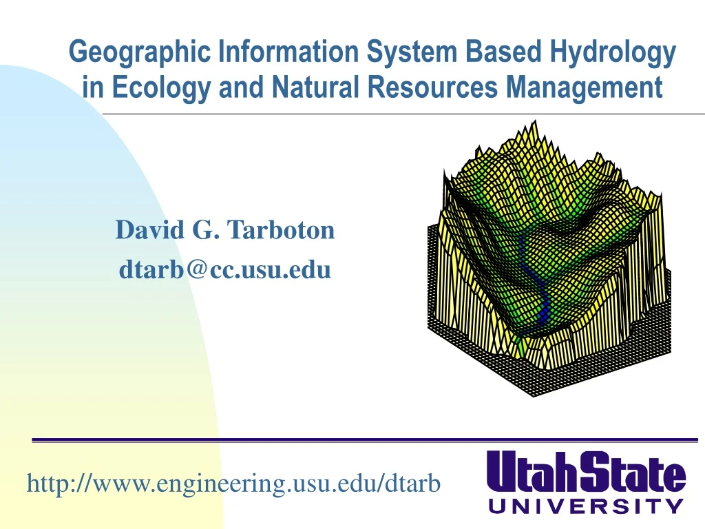
Geographic Information System Based Hydrology in Ecology and Natural Resources Management

1. Geographic Information System Based Hydrology in Ecology and Natural Resources Management David G. Tarboton dtarb@cc.usu.edu http://www.engineering.usu.edu/dtarb

2. Overview • Channel and watershed delineation • Hydrologic modeling (Bandaragoda) • Terrain stability mapping and erosion (Goodwin, Pack, Istanbulluoglu) • Dryland vegetation, a moisture limited ecological continuum (Goodwin) • Vegetation disturbance sediment model (Istanbulluoglu)

3. Hydrologic processes are different on hillslopes and in channels. It is important to recognize this and account for this in models. Objective delineation of channel networks using digital elevation models Drainage area can be concentrated or dispersed (specific catchment area) representing concentrated or dispersed flow.

4. DEM based channel network delineation using local curvature and constant drop analysis to have objective and spatially variable drainage density Eight direction pour point model D8 4 3 2 1 5 6 7 1 1 1 1 8 1 3 43 48 48 51 51 56 Threshold = 20 Dd = 1.9 km-1 t = -1.03 41 47 47 54 54 58 4 16 Threshold = 10 Dd = 2.5 km-1 t = -3.5 4 Flow direction network Accumulation of "valley" cells Local Valley Computation(Peuker and Douglas, 1975, Comput. Graphics Image Proc. 4:375) Stream drop test for highest resolution network (smallest threshold) with constant drop property satisfied, i.e. t test indicates no statistically significant difference in mean drop between first order and all higher order streams.

5. Curvature based stream delineation with threshold by constant drop analysis

6. 100 grid cell constant drainage area threshold stream delineation

7. 200 grid cell constant drainage area based stream delineation

8. Model Element Spatial Resolution Baron subwatersheds from streams delineated using objectively estimated drainage density from constant drop analysis. Baron subwatersheds generalized based on third order streams.

9. ? Topographic Slope Topographic Definition Drop/Distance Limitation imposed by 8 grid directions. Flow Direction Field — if the elevation surface is differentiable (except perhaps for countable discontinuities) the horizontal component of the surface normal defines a flow direction field.

10. The D Algorithm Tarboton, D. G., (1997), "A New Method for the Determination of Flow Directions and Contributing Areas in Grid Digital Elevation Models," Water Resources Research, 33(2): 309-319.) (http://www.engineering.usu.edu/cee/faculty/dtarb/dinf.pdf)

11. Contributing Area using D Contributing Area using D8

12. Useful for example to track where sediment or contaminant moves

13. Useful for example to track where a contaminant may come from

14. Useful for a tracking contaminant or compound subject to decay or attenuation

15. Transport limited accumulation Useful for modeling erosion and sediment delivery, the spatial dependence of sediment delivery ratio and contaminant that adheres to sediment

16. Reverse Accumulation Useful for destabilization sensitivity in landslide hazard assessment with Bob Pack

17. SINMAP Terrain Stability Mapping ArcView 3.x Extension (Bob Pack, Craig Goodwin)

18. Saturated Zone State Variable • Soil moisture deficit/depth to water table from wetness index determines saturated area • Baseflow response from average soil moisture deficit Local soil moisture enhancement If z < zr SR is enhanced locally to TOPNET • Enhanced TOPMODEL (Beven and Kirkby, 1979 and later) applied to each subwatershed model element. • Kinematic wave routing of subwatershed inputs through stream channel network. • Vegetation based interception component. • Modified soil zone • Infiltration excess • GIS based parameterization • (TOPSETUP) Reference ET demand Priestly-Taylor temp. and radiation based Interception Store Canopy Capacity CC (m) Canopy Storage CV (m) Throughfall Snow (in progress) Precipitation Infiltration capacity zr Soil Store SR(m) =Soil Zone water content Infiltration Excess Runoff Zr=depth of root zone z Soil Zone Drainage Precipitation Saturation Excess Runoff Streamflow Baseflow With Christina Bandaragoda

19. Wetness index histogram for each subwatershed used to parameterize subgrid variability of soil moisture Basin 1 Basin 2 Basin 3 0.20 0.20 0.20 0.15 0.10 Proportion of area Proportion of area Proportion of area 0.10 0.10 0.05 0.00 0.00 0.00 0 5 10 15 20 0 5 10 15 20 25 0 5 10 15 20 ln(a/S) (a in meter units) ln(a/S) (a in meter units) ln(a/S) (a in meter units) Basin 4 0.30 0.20 Proportion of area Basin 6 0.10 0.00 0.20 0 5 10 15 20 ln(a/S) (a in meter units) Proportion of area 0.10 0.00 Basin 9 0 5 10 15 20 ln(a/S) (a in meter units) 0.20 Basin 7 Basin 8 0.15 Proportion of area 0.10 0.20 0.20 0.05 Proportion of area Proportion of area 0.10 0.10 0.00 0 5 10 15 20 ln(a/S) (a in meter units) 0.00 0.00 0 5 10 15 20 0 5 10 15 20 ln(a/S) (a in meter units) ln(a/S) (a in meter units) With Christina Bandaragoda

20. q1 ,, q2 , &yf f & K … STATSGO Soil derived parameters Soil texture for each of the 11 standard soil depth grid layers from PSU gridding of NRCS STATSGO data. Zone Code Polygon Layer Depth weighted average Soil Grid Layers Joined to Polygon Layer Exponential decrease with depth Soil parameter look up by zone code Table of Soil Hydraulic Properties – Clapp Hornberger 1978 With Christina Bandaragoda

21. Basin average precipitation Streamflow at outlet Cumulativewater balance

22. “White space” is the Grey at Dobson minus Ahaura, Arnold and Grey at Waipuna

23. Shear Stress Threshold Model for Channel Initiation Channels incise when; tftc tf: Effective Shear Stress Overland Flow; • Overland flow, qo; • Contributing area, a • Excess rainfall rate, r • Roughness, n; • Bare soil, or grains, nb(d50) • Additional roughness, na • Slope, S • tc :Critical Shear Stress • -Sediment Size, d50 • -Dimensionless Critical Shear Stress, t* With Erkan Istanbulluoglu, Bob Pack, Charlie Luce

24. The PCI Theory • Hydraulic and hydrologic hillslope properties are treated as random variables with spatially homogenous probability distributions. With Erkan Istanbulluoglu, Bob Pack, Charlie Luce

25. Field observations • Channel head locations identified • Local slopes estimated in the field. • Contributing areas were derived from the DEM. • Sediment size samples were collected just above the headcuts. • Gully cross-section areas measured. With Erkan Istanbulluoglu, Bob Pack, Charlie Luce

26. With Erkan Istanbulluoglu, Bob Pack, Charlie Luce

27. Point-wise Comparison of the Observed aSa and Calculated C at Channel Heads • The theory developed suggested that variation in d50, na and r is responsible for the variation in aS at channel heads. We used the measured values of d50 to test the contribution of d50 to this variability. We set =1.167, r = 35 mm/h, na= 0.052. The regression R2 and Nash-Sutcliff (NS) error measure indicate that about 40% of the variability in observed aS may be attributed to d50. R2=0.387 NS=0.377 With Erkan Istanbulluoglu, Bob Pack, Charlie Luce

28. Comparison of Channel Initiation Probability Distributions Trapper Creek Data With Erkan Istanbulluoglu, Bob Pack, Charlie Luce

29. PCI in Slope-Area Diagrams With Erkan Istanbulluoglu, Bob Pack, Charlie Luce

30. Comparison of Channel Initiation Probability Distributions • Tennessee valley data set (Montgomery and Dietrich, 1989;1992). With Erkan Istanbulluoglu, Bob Pack, Charlie Luce

31. PCI Maps of the Study Watersheds With Erkan Istanbulluoglu, Bob Pack, Charlie Luce

32. Field Estimates of Transport Capacity • Gully cross-sections are surveyed at • 20-30 m spacing. • Slope of each segment is measured. • Sediment volumes are accumulated • downslope. Tr. 18 Tr. 15 Tr. 5 Tr. 19 With Erkan Istanbulluoglu, Bob Pack, Charlie Luce

33. Field Data; With Erkan Istanbulluoglu, Bob Pack, Charlie Luce

34. as a function of With Erkan Istanbulluoglu, Bob Pack, Charlie Luce

35. Craig Goodwin Dryland Vegetation Distribution Basic Premises • Moisture is the most significant resource limitation in drylands • Topography is a major factor regulating landscape moisture by: • Redistribution of moisture by overland flow • No subsurface lateral flow • Solar radiation exposure • South slope versus north slope

36. Topographic Factors Craig Goodwin Solar Radiation Exposure South-facing Hillslope North-facing Hillslope Moisture Redistribution

37. Craig Goodwin Ecological field data collection • Cover data collected at approximately 60 transects (30 m long) per watershed. • Cover data collected for 100 points per transect, by species, using the “point intercept on a transect method.”

38. Craig Goodwin

39. Craig Goodwin Hydrology Component: Basis • Landscape moisture in drylands is derived from infiltration of precipitation (ip) and overland flow runon (iq). • Infiltration and runoff (q) are partitioned using a storage threshold (h) concept. Daily (storm) rainfalls (p) are derived from an exponential distribution. Total average annual runoff at a point (qa) is obtained by summing over the distribution of precipitation days. [Kirkby, 1994] • A fraction of runon (qin) infiltrates at a point. The fraction that infiltrates is a function of discharge and surface characteristics (ks), which control time of overland flow occurrence at that point. • Large bare ground expanses reduce soil moisture through evaporation. Currently, evaporation is estimated by a simple expression involving climate (kc) and solar radiation (R) parameters (kr), but more robust methods could be used. • A landscape moisture index (LMI), which is spatially distributed across a dryland landscape, is the end product of the hydrology component.

40. Craig Goodwin Landscape Moisture Index Distribution of the landscape moisture index (LMI) across Kendall watershed. Transects average the LMI cell values of cells that they intersect, and are binned into four categories that match the LMI categories. The very dry sites are on the south facing slopes, whereas dry sites occur on north facing slopes. The damp and moist categories occur along the mainstem valley and the two major tributary valleys. Note how the LMI incorporates characteristics of solar radiation and overland flow discharge (and specific catchment area). In the table to the right, vegetation cover data are ordered by LMI and binned using the same categories as shown on the map above. Cover and LMI data for 4 Species at 55 transects. Cover is number of species hits out of a possible 100.

41. Craig Goodwin Cover Frequency Chart This graph illustrates the binned field data presented in the table on the previous slide. Only four of the 20 species in the watershed are illustrated. These data were used to predict species distribution across the landscape. Distribution of black gramma and velvet mesquite are illustrated on the next slide.

42. Craig Goodwin Species Distribution Mesquite distribution based upon LMI. Black gramma distribution based upon LMI.

43. Craig Goodwin Other Potential Indices:Do They Work As Well?

44. Erkan Istanbulluoglu • Vegetation Disturbance Sediment Model • Purposes • How do forest cover conditions influence the frequency and magnitude of stream sediment inputs. • How do natural and human disturbances alter these frequencies and magnitudes. • Motivated by biologic and aquatic community dependence on sediment input regime.

45. MODELING APPROACH Erkan Istanbulluoglu

46. Erkan Istanbulluoglu Recovery Following Wildfires • In the first few years following vegetation loss fluvial erosion is often observed during thunderstorms. • Following the initial significant increase erosion is suppressed by the growth of under-story vegetation and recovery of the infiltration rates (in 3 to 5 yrs) • Root-strength reduces to minimum values usually after 10 – 15 years and increases landslide susceptibility during this period.

47. FOREST FIRES Sampled Annual Maximum Rainfall Runoff Response Vegetation Response 10000 years simulation Erosive Response Erkan Istanbulluoglu

48. Erkan Istanbulluoglu CONSTANT ROOT COHESION (No Vegetation Disturbance) Soil depth at a point Summary of the simulations

49. 95% Quantile Modeled EventS.Y. Event S.Y. (Observed) 8% Quantile Modeled LASY LASY (Observed) SASY (Observed)

50. AREA 2 3 AREA 1 Are there any questions ? 12 Conclusion • Spatial hydrologic processes play a key role in integrating hydrology with to other fields including Geomorphology, Ecology, and Environmental Policy and Management http://www.engineering.usu.edu/dtarb