Download
1 / 99
1k likes | 1.1k Vues
This text delves into structured prediction techniques using perceptrons and conditional random fields (CRFs) in the context of Natural Language Processing (NLP). It covers topics such as finding the best outputs given inputs and implementing probabilistic parsing. The course discusses weighted CKY algorithms, probability distributions, and maximizing joint probabilities for various NLP tasks like speech recognition, machine translation, and parsing. It explores the intersection of linguistics and probability in modeling linguistic objects, syntax, and semantics quantitatively. The text also touches on non-probabilistic methods like transfer-based learning and competitive linking. Overall, it provides an overview of structured prediction and its applications in NLP.

E N D
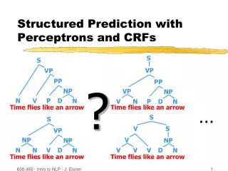
S S VP VP PP PP VP NP NP N V P D V N P D N N S S V S VP NP V NP NP N N V D V V V D N N Structured Prediction with Perceptrons and CRFs ? Time flies like an arrow Time flies like an arrow … Time flies like an arrow Time flies like an arrow 600.465 - Intro to NLP - J. Eisner
Structured Prediction with Perceptrons and CRFs But now, modelstructures! Back to conditionallog-linear modeling … 600.465 - Intro to NLP - J. Eisner 2
p(fill | shape) 600.465 - Intro to NLP - J. Eisner 3
p(fill | shape) 600.465 - Intro to NLP - J. Eisner 4
p(category | message) goodmail spam Reply today to claim your … Reply today to claim your … goodmail spam Wanna get pizza tonight? Wanna get pizza tonight? goodmail spam Thx; consider enlarging the … Thx; consider enlarging the … goodmail spam Enlarge your hidden … Enlarge your hidden …
p(RHS | LHS) S NP VP S S NP[+wh] V S/V/NP N VP … PP P Det N S S S VP NP 600.465 - Intro to NLP - J. Eisner 6
p(RHS | LHS) S NP VP S S NP[+wh] V S/V/NP N VP … PP P Det N S S S VP NP NP NP VP NP NP NP CP/NP N VP … NP PP Det N NP NP NP VP NP … 600.465 - Intro to NLP - J. Eisner 7
p(parse | sentence) Time flies like an arrow Time flies like an arrow … Time flies like an arrow Time flies like an arrow 600.465 - Intro to NLP - J. Eisner 8
p(tag sequence | word sequence) Time flies like an arrow Time flies like an arrow … Time flies like an arrow Time flies like an arrow 600.465 - Intro to NLP - J. Eisner 9
Today’s general problem • Given some input x • Occasionally empty, e.g., no input needed for a generative n-gram or model of strings (randsent) • Consider a set of candidate outputs y • Classifications for x (small number: often just 2) • Taggings of x (exponentially many) • Parses of x (exponential, even infinite) • Translations of x (exponential, even infinite) • … • Want to find the “best” y, given x Structured prediction 600.465 - Intro to NLP - J. Eisner
Remember Weighted CKY …(find the minimum-weight parse) 1 S NP VP 6 S Vst NP 2 S S PP 1 VP V NP 2 VP VP PP 1 NP Det N 2 NP NP PP 3 NP NP NP 0 PP P NP 11
But is weighted CKY good for anything else?? multiply to get 2-22 2-2 2-8 2-12 So far, we used weighted CKY only to implement probabilistic CKY for PCFGs 1 S NP VP 6 S Vst NP 2 S S PP 1 VP V NP 2 VP VP PP 1 NP Det N 2 NP NP PP 3 NP NP NP 0 PP P NP 12
But is weighted CKY good for anything else?? Do the weights have to be probabilities? We set the weights to log probs S NP time VP | S) = w(S NP VP) + w(NP time) w( PP VP flies P like NP + w(VP VP NP) Det an N arrow + w(VP flies) + … Just let w(X Y Z) = -log p(X Y Z| X) Then lightest tree has highest prob 13
summary of half of the course (statistics) Probability is Useful • We love probability distributions! • We’ve learned how to define & use p(…) functions. • Pick best output text T from a set of candidates • speech recognition (HW2); machine translation; OCR; spell correction... • maximize p1(T) for some appropriate distribution p1 • Pick best annotation T for a fixed input I • text categorization; parsing; part-of-speech tagging … • maximize p(T | I); equivalently maximize joint probability p(I,T) • often define p(I,T) by noisy channel: p(I,T) = p(T) * p(I | T) • speech recognition & other tasks above are cases of this too: • we’re maximizing an appropriate p1(T) defined by p(T | I) • Pick best probability distribution (a meta-problem!) • really, pick best parameters: train HMM, PCFG, n-grams, clusters … • maximum likelihood;smoothing;EM if unsupervised (incomplete data) • Bayesian smoothing: max p(|data) = max p(, data) =p()p(data|) 600.465 - Intro to NLP - J. Eisner
summary of other half of the course (linguistics) Probability is Flexible • We love probability distributions! • We’ve learned how to define & use p(…) functions. • We want p(…) to define probability of linguistic objects • Trees of (non)terminals (PCFGs; CKY, Earley, pruning, inside-outside) • Sequences of words, tags, morphemes, phonemes (n-grams, FSAs, FSTs; regex compilation, best-paths, forward-backward, collocations) • Vectors (decis.lists, Gaussians, naïve Bayes; Yarowsky, clustering/k-NN) • We’ve also seen some not-so-probabilistic stuff • Syntactic features, semantics, morph., Gold. Could be stochasticized? • Methods can be quantitative & data-driven but not fully probabilistic: transf.-based learning, bottom-up clustering, LSA, competitive linking • But probabilities have wormed their way into most things • p(…) has to capture our intuitions about the ling. data 600.465 - Intro to NLP - J. Eisner
An Alternative Tradition • Old AI hacking technique: • Possible parses (or whatever) have scores. • Pick the one with the best score. • How do you define the score? • Completely ad hoc! • Throw anything you want into the stew • Add a bonus for this, a penalty for that, etc. 600.465 - Intro to NLP - J. Eisner
Scoring by Linear Models Weight of feature k (learned or set by hand) Whether (x,y) has feature k(0 or 1) Or how many times it fires ( 0) Or howstrongly it fires (real #) Ranges over all features, e.g., k=5 (numbered features)or k=“see Det Noun” (named features) • Given some input x • Consider a set of candidate outputs y • Define a scoring functionscore(x,y) Linear function: A sum of feature weights (you pick the features!) • Choose y that maximizes score(x,y) 600.465 - Intro to NLP - J. Eisner 17
Scoring by Linear Models (learned or set by hand) This linear decision rule is sometimes called a “perceptron.” It’s a “structured perceptron” if it does structured prediction (number of y candidates is unbounded, e.g., grows with |x|). • Given some input x • Consider a set of candidate outputs y • Define a scoring functionscore(x,y) Linear function: A sum of feature weights (you pick the features!) • Choose y that maximizes score(x,y) 600.465 - Intro to NLP - J. Eisner 18
An Alternative Tradition Old AI hacking technique: Possible parses (or whatever) have scores. Pick the one with the best score. How do you define the score? Completely ad hoc! Throw anything you want into the stew Add a bonus for this, a penalty for that, etc. “Learns” over time – as you adjust bonuses and penalties by hand to improve performance. Total kludge, but totally flexible too … Can throw in any intuitions you might have Could we make it learn automatically? 600.465 - Intro to NLP - J. Eisner 19
Perceptron Training Algorithm • initialize θ (usually to the zero vector) • repeat: • Pick a training example (x,y) • Model predicts y* that maximizes score(x,y*) • Update weights by a step of size ε > 0:θ = θ + ε∙ (f(x,y) – f(x,y*)) If model prediction was correct (y=y*), θ doesn’t change. So once model predicts all training examples correctly, stop. If some θ can do the job, this eventually happens! (If not, θ will oscillate, but the averageθ from all stepswill settle down. So return that eventual average.)
Perceptron Training Algorithm • initialize θ (usually to the zero vector) • repeat: • Pick a training example (x,y) • Model predicts y* that maximizes score(x,y*) • Update weights by a step of size ε > 0:θ = θ + ε∙ (f(x,y) – f(x,y*)) If model prediction was wrong (y≠y*), then we must havescore(x,y) ≤ score(x,y*) instead of > as we want. Equivalently, θ∙f(x,y) ≤ θ∙f(x,y*) Equivalently, θ∙(f(x,y) - f(x,y*)) ≤ 0 but we want it positive. Our update increases it (by ε∙ || f(x,y) – f(x,y*) ||2≥ 0)
p(parse | sentence) score(sentence, parse) Time flies like an arrow Time flies like an arrow … Time flies like an arrow Time flies like an arrow 600.465 - Intro to NLP - J. Eisner 22
Finding the best y given x • At both training & test time, given input x, perceptron picks y that maximizes score(x,y) • How do we compute that crucial prediction?? • Easy when only a few candidates y(text classification, WSD, …) • Just try each y in turn. • Harder for structured prediction: but you now know how! • Find the best string, path, or tree … • That’s what Viterbi-style or Dijkstra-style algorithms are for. • That is, use dynamic programming to find the score of the best y. • Then follow backpointers to recover the y that achieves that score. 600.465 - Intro to NLP - J. Eisner 23
really so alternative? An Alternative Tradition Old AI hacking technique: Possible parses (or whatever) have scores. Pick the one with the best score. How do you define the score? Completely ad hoc! Throw anything you want into the stew Add a bonus for this, a penalty for that, etc. “Learns” over time – as you adjust bonuses and penalties by hand to improve performance. Total kludge, but totally flexible too … Can throw in any intuitions you might have Exposé at 9 Probabilistic RevolutionNot Really a Revolution, Critics Say Log-probabilities no more than scores in disguise “We’re just adding stuff up like the old corrupt regime did,” admits spokesperson 600.465 - Intro to NLP - J. Eisner 24
Nuthin’ but adding weights n-grams: … + log p(w7 | w5, w6) + log p(w8 | w6, w7) + … PCFG: log p(NP VP | S) + log p(Papa | NP) + log p(VP PP | VP) … HMM tagging: … + log p(t7 | t5, t6) + log p(w7 | t7) + … Noisy channel: [log p(source)] + [log p(data | source)] Cascade of composed FSTs: [log p(A)] + [log p(B | A)] + [log p(C | B)] + … Naïve Bayes: log p(Class) + log p(feature1 | Class) + log p(feature2 | Class) … Note: Here we’re using +logprob not –logprob:i.e., bigger weights are better. 600.465 - Intro to NLP - J. Eisner 25
Nuthin’ but adding weights n-grams: … + log p(w7 | w5, w6) + log p(w8 | w6, w7) + … PCFG: log p(NP VP | S) + log p(Papa | NP) + log p(VP PP | VP) … Score of a parse is its total weight The weights we add up have always been log-probs ( 0) but what if we changed that? HMM tagging: … + log p(t7 | t5, t6) + log p(w7 | t7) + … Noisy channel: [log p(source)] + [log p(data | source)] Cascade of FSTs: [log p(A)] + [log p(B | A)] + [log p(C | B)] + … Naïve Bayes: log(Class) + log(feature1 | Class) + log(feature2 | Class) + … 600.465 - Intro to NLP - J. Eisner 26
What if our weights were arbitrary real numbers? n-grams: … + log p(w7 | w5, w6) + log p(w8 | w6, w7) + … PCFG: log p(NP VP | S) + log p(Papa | NP) + log p(VP PP | VP) … HMM tagging: … + log p(t7 | t5, t6) + log p(w7 | t7) + … Noisy channel: [log p(source)] + [log p(data | source)] Cascade of FSTs: [log p(A)] + [log p(B | A)] + [log p(C | B)] + … Naïve Bayes: log p(Class) + log p(feature1 | Class) + log p(feature2 | Class) … Change log p(this | that) to (this; that) 600.465 - Intro to NLP - J. Eisner 27
What if our weights were arbitrary real numbers? n-grams: … + (w7 ; w5, w6) + (w8 ; w6, w7) + … PCFG: (NP VP ; S) + (Papa ; NP) + (VP PP ; VP) … HMM tagging: … + (t7 ; t5, t6) + (w7 ; t7) + … Noisy channel: [ (source)] + [ (data ; source)] Cascade of FSTs: [ (A)] + [ (B ; A)] + [ (C ; B)] + … Naïve Bayes:(Class) + (feature1 ; Class) + (feature2 ; Class) … Change log p(this | that) to (this ; that) In practice, is a hash table Maps from feature name(a string or object) to feature weight(a float) e.g., (NP VP ; S) = weight of the S NP VP rule, say -0.1or +1.3 600.465 - Intro to NLP - J. Eisner 28
What if our weights were arbitrary real numbers? n-grams: … + (w5 w6 w7) + (w6 w7 w8) + … PCFG: (S NP VP) + (NP Papa) + (VP VP PP) … HMM tagging: … + (t5 t6 t7) + (t7 w7) + … Noisy channel: [ (source)] + [ (source, data)] Cascade of FSTs: [ (A)] + [ (A, B) ] + [ (B, C)] + … Naïve Bayes:(Class) + (Class, feature 1) + (Class, feature2) … Change log p(this | that) to (this ; that) (that & this) [prettiername] WCFG (multi-class) logistic regression In practice, is a hash table Maps from feature name(a string or object) to feature weight(a float) e.g., (S NP VP) = weight of the S NP VP rule, say -0.1or +1.3 600.465 - Intro to NLP - J. Eisner 29
What if our weights were arbitrary real numbers? n-grams: … + (w5 w6 w7) + (w6 w7 w8) + … Best string is the one whose trigrams have the highest total weight PCFG: (S NP VP) + (NP Papa) + (VP VP PP) … Best parse is one whose rules have highest total weight HMM tagging: … + (t5 t6 t7) + (t7 w7) + … Best tagging has highest total weight of all transitions and emissions Noisy channel: [ (source)] + [ (source, data)] To guess source: max (weight of source + weight of source-data match) Naïve Bayes:(Class) + (Class, feature 1) + (Class, feature 2) … Best class maximizes prior weight + weight of compatibility with features Change log p(this | that) to (that & this) WCFG (multi-class) logistic regression 600.465 - Intro to NLP - J. Eisner 30
What if our weights were arbitrary real numbers? n-grams: … + (w5 w6 w7) + (w6 w7 w8) + … Best string is the one whose trigrams have the highest total weight PCFG: (S NP VP) + (NP Papa) + (VP VP PP) … Best parse is one whose rules have highest total weight (use CKY/Earley) HMM tagging: … + (t5 t6 t7) + (t7 w7) + … Best tagging has highest total weight of all transitions and emissions Noisy channel: [ (source)] + [ (source, data)] To guess source: max (weight of source + weight of source-data match) Naïve Bayes:(Class) + (Class, feature 1) + (Class, feature 2) … Best class maximizes prior weight + weight of compatibility with features Change log p(this | that) to (that & this) All our algorithms still work! We’ll just add up arbitrary feature weights θ that might not be log conditional probabilities (they might even be positive!) Total score(x,y) can’t be interpretedanymore as log p(x,y) But we can still find the highest-scoring y WCFG (multi-class) logistic regression 600.465 - Intro to NLP - J. Eisner 31
S VP PP NP N N V P D Time flies like an arrow Given sentencex You know how to find max-score parsey (or min-cost parse as shown) • Provided that the score of a parse = total score of its rules 1 S NP VP 6 S Vst NP 2 S S PP 1 VP V NP 2 VP VP PP 1 NP Det N 2 NP NP PP 3 NP NP NP 0 PP P NP
Given word sequencex You know how to find max-score tag sequence y • Provided that the score of a tagged sentence = total score of its emissions and transitions • These don’t have to be log-probabilities! • Emission scores assess tag-word compatibility • Transition scores assess goodness of tag bigrams …? Prep Adj Verb Verb Noun Verb PN Adj Det Noun Prep Noun Prep Det Noun Bill directed a cortege of autos through the dunes
Given upper stringx You know how to find max-score path that accepts x (or min-cost path) • Provided that the score of a path = total score of its arcs • Then the best lower string y is the one along that best path • (So in effect, score(x,y) is score of best path that transduces x to y) • Q: How do you make sure that the path accepts x, such as aaaaaba? • A: Compose with straight-line automaton for x, then find best path.
Why would we switch from probabilities to scores? • “Discriminative” training (e.g., perceptron) might work better. • It tries to optimize weights to actually predict the right y for each x. • More important than maximizing log p(x,y) = log p(y|x) + log p(x),as we’ve been doing in HMMs and PCFGs. • Satisfied once the right y wins. The example puts no more pressure on the weights to raise log p(y|x). And never pressures us to raise log p(x). • Having more freedom in the weights might help? • Now weights can be positive or negative. • Exponentiated weights no longer have to sum to 1. • But turns out new θ vectors can’t do more than the old restricted ones. • Roughly, for every WCFG there’s an equivalent PCFG. • Though it’s true a regularizer might favor one of the new ones. • We can throw lots more features into the stewpot. • Allows model to capture more of the useful predictive patterns! • So, what features can we throw in efficiently?
When can you efficiently choose best y? e.g, θ3 = score of VP VP PP f3(x,y) = # times VP VP PPappears in y • “Provided that the score of a parse = total score of its rules” • “Provided that the score of a tagged sentence = total score of its transitions and emissions” • “Provided that the score of a path = total score of its arcs” This implies certain kinds of features in linear model … 600.465 - Intro to NLP - J. Eisner 36
When can you efficiently choose best y? • “Provided that the score of a parse = total score of its rules” • “Provided that the score of a tagged sentence = total score of its transitions and emissions” • “Provided that the score of a path = total score of its arcs” This implies certain kinds of features in linear model … More generally: make a list of interesting substructures. The feature fk(x,y) counts tokens of kth substructure in (x,y). So far, the substructures = the grammar rules (for a PCFG). But model could use any features … what ones are efficient? 600.465 - Intro to NLP - J. Eisner 37
S VP PP NP VP NP N V P D N 1. Single-rule substructures • Count of VP VP PP Time flies like an arrow
S VP PP NP VP NP N V P D N 1. Single-rule substructures • Count of VP VP PP • Count of V flies These features are efficient for CKY to consider. Time flies like an arrow (looks at y only) (looks at both x and y)
S VP PP NP VP NP N V P D N 2. Within-rule substructures • Count of VP with a PP child Time flies like an arrow
S VP PP NP VP NP N V P D N 2. Within-rule substructures • Count of VP with a PP child • Count of any node with a PP right child Time flies like an arrow
S VP PP NP VP NP N V P D N 2. Within-rule substructures • Count of VP with a PP child • Count of any node with a PP right child • Count of any node with a PP right child and whose label matches left child’s label Time flies like an arrow
S VP PP NP VP NP N V P D N 2. Within-rule substructures Efficient?Yes: the weight that CKY uses for VP VP PP is the total weight of all of its within-rule features. • Count of VP with a PP child • Count of any node with a PP right child • Count of any node with a PP right child and whose label matches left child’s label Some of these features fire on both VP VP PP and NP NP PP. So they’re really backoff features. Time flies like an arrow
S VP PP NP VP NP N V P D N 3. Cross-rule substructures • Count of “flies” as a verb with subject “time” Time flies like an arrow
S VP PP NP VP NP N V P D N 3. Cross-rule substructures • Count of “flies” as a verb with subject “time” • Count of NP D N when the NP is the object of a preposition Time flies like an arrow
S Two such VPs, so feature fires twice on this (x,y) pair VP PP NP VP NP N V P D N 3. Cross-rule substructures • Count of “flies” as a verb with subject “time” • Count of NP D N when the NP is the object of a preposition • Count of VPs that contain a V Time flies like an arrow
S VP PP NP VP NP N V P D N 3. Cross-rule substructures Efficient? Sort of.For CKY to work, must add attributes to the nonterminals so that these features can now be detected within-rule. That enlarges the grammar. • Count of “flies” as a verb with subject “time” • Count of NP D N when the NP is the object of a preposition • Count of VPs that contain a V [hasV=true] [head=time] [hasV=true] [role=prepobj] Time flies like an arrow What’s the analogue in FSMs? Splitting states to remember more history.
S VP PP NP VP NP N V P D N 4. Global features • Count of “NP and NP” when the two NPs have very different size or structure [this feature has weight < 0] • The number of PPs is even • The depth of the tree is prime • Count of the tag bigram V P in the preterminal seq Time flies like an arrow
S [depth=5] VP [depth=4] PP NP VP [depth=3] NP [depth=2] [depth=2] [depth=2] N V P D N [depth=1] [depth=1] [depth=1] [depth=1] 4. Global features Efficient? Depends on whether you can do it with attributes. If you have infinitely many nonterminals, it’s not technically a PCFG anymore, but CKY might still apply. Or stop relying only on dynamic programming. Start using approximate or exact general methods for combinatorial optimization. Hot area! • Count of “NP and NP” when the two NPs have very different size or structure [this feature has weight < 0] • The number of PPs is even • The depth of the tree is prime • Count of the tag bigram V P in the preterminal seq Time flies like an arrow
S VP PP NP VP NP N V P D N 5. Context-specific features Take any efficient feature that counts a substructure. Modify it to count only tokens appearing in a particular red context. Time flies like an arrow